읽는 배경 : Recognition Basic. Understand confusing and ambiguous things.
읽으면서 생각할 포인트 : 코드와 함께 최대한 완벽히 이해하기. 이해한 것 정확히 기록해두기.
느낀점 :
최근 논문일수록, 블로그나 동영상의 내용 정리가 두리뭉실하고 이해하기 힘들다. 디테일성은 거의 없다. 따라서 그냥 논문 읽는게 최고다. 만약 블로그에 내용 정리가 잘 되어 있다고 하더라도, 내가 블로그 내용에 대한 신뢰가 안가서, 합리적 추론의 이해(덜 디테일한 설명은 나의 생각을 좀 더 추가해서 이해하는 과정)을 할 수도 없다. 따라서 논문이나 읽자. 시간 낭비하지 말고.
SSD 코드를 공부했을때 모듈화가 심각해서 보기가 힘들었다. 하지만 그것은 “처음부터 끝까지 다 봐야지.” 라는 욕심때문에 보기 힘들었던 것 같다. 하지만 사실 그렇게 코드를 보는 경우는 드믄것 같다. “내가 궁금한 부분만 찾아보거나, 내가 사용하고 싶은 모듈만 찾아서 사용한다.”라는 마음으로 부분 부분 코드를 본다면, 내가 원하는 부분을 전체 코드에서 찾는 것은 그리 어렵지 않다. 라는 것을 오늘 느꼈다.
블로그 : 너무 result 해석에 많은 초점을 둔다. 방법론에 대해서는 구체적이지는 않아, 나에게는 이해가 어려웠다. 논문이나 읽자.
동영상 : 핵심이 Casecade-Mask RCNN이다. 디테일이 거의 없다. 안봄.
참고자료 내용 정리 :
이 논몬은 object detector의 약점을 잘 파악했다. 이 논문을 통해, 아주 복잡한 방법을 적용해서 성능 향상을 미약하게 이루는 것 보다는, 문제점을 잘 파악하기만 하면 어렵지 않게 성능을 향상시킬 수 있음을 보여준다.
문제점 파악하기
Introduction에 실험 그래프가 나온다. 블로그 글은 이해 안되서, 논문 읽는게 낫겠다.
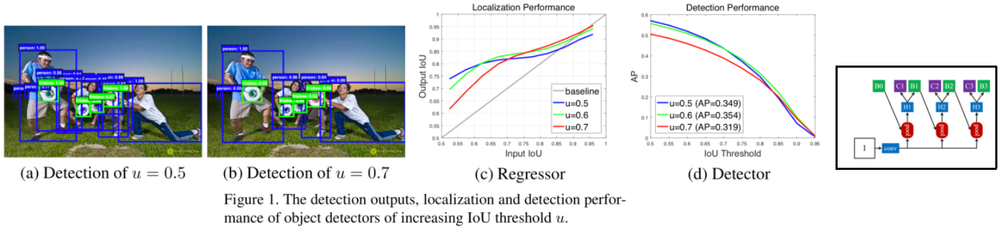
Cascade R-CNN은 위 사진의 오른쪽 그림의 구조이다. 굳이 설명하지 않겠다. 특히 단계를 거듭할 수록 보다 더 높은 IOU를 기준으로 학습시킨다.
과거 방식 (1) 단순하게 하나의(같은) classifier를 Iterative하게 사용하는 것은 큰 성능 향상을 주지 못한다. (2) 서로 다른 classifier를 여러개 만들고, 각각의 IOU기준을 다르게 주고 학습을 시키는 방법도 성능 향상은 그저 크지 않다. 즉 여러 classifier의 ensenble 방법이다.
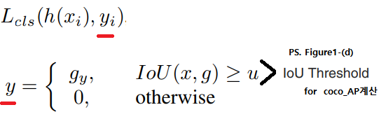
Cascade R-CNN은 각각의 classifier는 각각 Threshold 0.5, 0.6, 0.7 로 학습. 예측 bounding box와 GT-box가 겹치는 정도가 Threshold 이상이여야지만, 옳게 예측한 것이라고 인정해줌. 이하라면 regressing 틀린거로 간주하고 loss를 준다.
크면 Positive Bounding box(당당하게 이건 객체다! 라고 말하는 예측 BB값),
작으면 Negative(Bounding Box이긴 하지만, 아무래도 이건 객체는.. 아니다. 라고 말하는 예측 BB값)
여기서 P, N이, [TP FP TN FN]에서 P, N 이다.
abstract, Introduction
현재 문제점들
close false positives = “close but not correct 거의 맞췄지만.. 아니야” bounding boxes 가 많기 때문에 더욱 어려운 문제이다.
통상적으로 우리는 IOU threshold = 0.5 를 사용합니다. 하지만 이것은 a loose requirement for positives (약간은 느슨한,쉬운 요구조건) 입니다. 따라서 detector는 자주 noise bounding box를 만들어 낸다. 이것 때문에 우리는 항상 reject close false positives 에 어려움을 더 격고 있다.
즉. 아래의 그림과 같이, u=0.5일 때.. Detected bounding box에 대해서 너무 약한 threshold를 주기 때문에 아래와 같은 noise스러운 박스들이 많이 추출 된다.
분석해보기
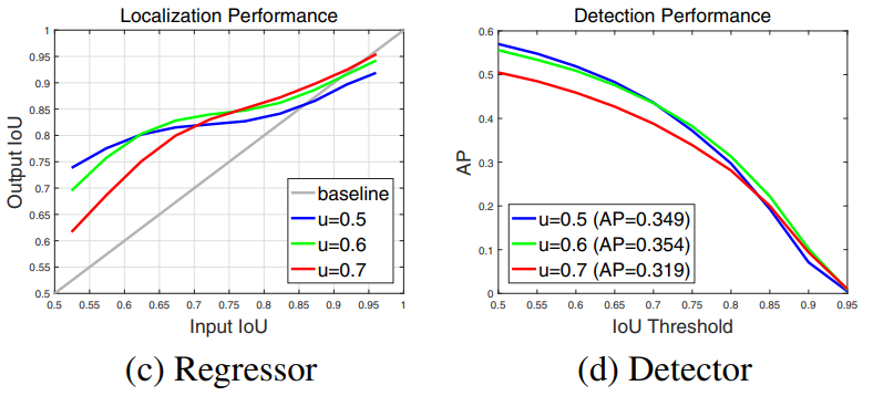
그림(c) : X : Input Proposal(RPN에서 나오는 BB와 GT), Y : detection performance(Classifier에서 오는 BB와 GT) u=0.7에서는 일정 이상의 X에서만 높은 Y값이 나온다.
그림(d) : u=0.5로 했을때(0.5이상은 모두 객체로 탐지. 모든 Positive들), Threshold(이 이상만 TP로 판단. 이 이외는 FP)가 어떤 때든 상대적으로 좋은 AP가 도출 된다.
( 일반적으로 이렇게 하나의 IOU값으로 최적화된 모델(Detector)은 다른 IOU threshold에서도 최적화된 값(Hypotheses=예측/추론값)이 나오기 힘들다. )
그렇다고 u를 그냥 높게 하는 건 좋지 않다. (d)에서 보이는 결과도 그렇고 Overfitting이 발생하는 경향도 있다. 또한 (c)에서 처럼 u=0.7에서는 일정 이상의 X에서만 높은 Y값이 나온다. 일정 이하는 그리.. 최적화된 신경망이 만들어 진다고 볼 수 없다.
이 논문의 저자는 생각했다. bounding box regressor를 0.5 ~ 0.6 ~ 0.7 의 u로 키워가며 stage를 거치게 하는 것은 (c)에서, 낮은 X에서는 파랑Line을, 중간 X에서는 초록Line을, 높은 X에서는 빨간Line이상의 값을 OutputIOU로 가지게 함으로써 적어도 회색 대각선보다는 높은 곳에 점이 찍히게 하는 것을 목표로 한다.
우리의 방법
나만의 직관적 이해 : ⭐⭐
만약 RPN에서 나온 BB와 GT간의 IOU가 0.55이고, Classifier에서 나온 BB와 GT간의 IOU가 0.58라고 해보자.(class는 맞았다고 가정)
만약 Threshold=0.6이라면, (클래스는 맞았음에도 불구하고 BB위치가 틀렸기 때문에) 이것은 FP라고 처리 된다.
이것이야 말로 close false positives 이다.
하지만 아까 0.58의 BB정보를 sequentially하게 옆의 Classifier에 넘겨주고 이 Classifier에서 나오는 BB와 GT간의 IOU가 0.61이 된다면!
이것은 완벽히 close false positives에 대한 문제를 해결해준 것이라고 할 수 있다.
Cascade R-CNN does not aim to mine hard negatives.(즉 클래스에 관점에서 AP를 높히는 것이 아니다.) Instead, by adjusting bounding boxes(Regressing 관점에서 AP를 높이려는 목표를 가진다.)
Related Work, Object Detection
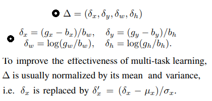
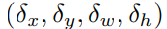
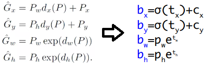
Offset Relative 공식 :
Figure 3 (b) : same classifier / 모두 u = 0.5 / 따라서 위의 그래프 (c)에서 보는 것처럼 u=0.5이고 X가 일정 이상일때 오히려 Y값이 더 낮아지는 현상을 간과 했다. / 또한 위 그림의 Figure2에서 보는 것처럼, (blue dot) 첫번째 stage에서 BB의 offset Relative로 인해 refine이 이뤄지지만, 두, 세번째 stage에서는 분산 값이 좁게 변한다. 초기에 이미 Optimal이라고 판단하는 듯 하다 /
Detection Quality
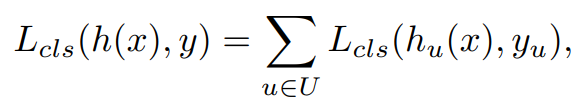
Figure3-(c) Integral Loss
U = {0.5, 0.55, ⋅⋅⋅ , 0.75}를 가지는 Classifier들을 모두 모두 모아서 Ensemble을 수생한다.
많은 Classifier가 있으므로, 이들에 대한 모든 Classifier Loss는 아래와 같다.
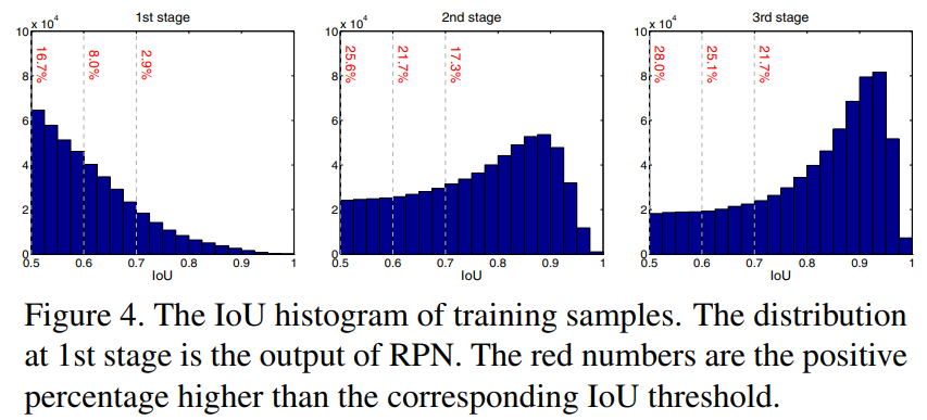
아래 Figure4의 첫번째 그래프를 보더라도, 0.7이상의 IOU를 가지는 BB는 2.9프로 밖에 안된다. 이래서 좋은 U를 가지는 Classifier는 빨리 Overfitting이 되버린다. 따라서 이러한 방법으로 close false positives문제가 해결되지는 않았다.
Cascade R-CNN
Cascaded Bounding Box Regression
4-3에서 blue dot에 대한 설명과 다르게 distribution이 1-stage와 비슷하게 유지되도록 노력했다. (그래서 나온 결과가 u=0.5, 0.6, 0.7)
는 normalized 된다. [Faster R-CNN] 널리 사용되는 방법이란다. 코드에서는 구체적인 normalization을 이루진 않았다. (필요하면! 아래의 아래 6-2 stat 부분 참조.)
Cascaded Detection
Experimental Results
Implementation Details
four stages : 1_RPN and 3_detection with U = {0.5, 0.6, 0.7}
horizontal image flipping 이외에 어떤 data augmentation도 사용되지 않았다.
Generalization Capacity
지금까지는 예측 BB의 GT와의 IOU를 증가시키려고 노력했다. 그럼 Figure(3)-d에서 C1,C2,C3는 어떻게 이용할까? 실험을 통해서 그냥 C3를 이용해서 Class 예측을 하는 것보다는, C1,C2,C3을 앙상블함으로써 더 좋은 AP를 얻어내었다고 한다.
(블로그 내용 참조 그리고 FasterRCNN논문도 나중에 참고해보기. 참고해봤는데 이런 내용 없다. 그래서 일단 블로그 작성자에게 “구체적으로 어디서 나온 내용이냐고” 질문 해봄. 질문이 잘 갔는지 모르겠다…) Regression Statistics = stat : 위의 offset relative 델타 값들은, Faster-RCNN에서 이 파라메터가 잘 나오게 학습시킬 때 L1 loss를 사용한다. 이때 델타값을 normalization하지 않으면 자칫 학습이 잘 이뤄지지 않는 문제가 있었다고 한다. 그래서 각 좌표값을 normalize하는 작업을 수행했다. (4-1의 수식처럼) 각 Stage에서 각자의 기준으로, regressing offset relative값에 대한 normalization을 수행했다는 의미인듯 하다.
Cascade 모듈은 다른 곳에서 쉽게 적용될 수 있다. 다른 기본 모델에 cacade모듈을 적용하여 효과적인 AP 상승을 이뤄낼 수 있었다고 한다.
# cascade-rcnn_Pytorch/lib/model/fpn/cascade/fpn.py
class_FPN(nn.Module):def__init__(self,classes,class_agnostic):self.RCNN_loss_cls=0self.RCNN_loss_bbox=0self.RCNN_rpn=_RPN_FPN(self.dout_base_model)self.RCNN_roi_align=RoIAlignAvg(cfg.POOLING_SIZE,cfg.POOLING_SIZE,1.0/16.0)# 다른 신경망을 봐야함 FPN에는 없음 아래 내용 2nd, 3rd에 동일 적용
self.RCNN_bbox_pred=nn.Linear(1024,4)self.RCNN_bbox_pred=nn.Linear(1024,4*self.n_classes)# 이게 u = 0.5, 0.6, 0.7 적용은 아래의 신경망이 사용된다.
self.RCNN_proposal_target=_ProposalTargetLayer(self.n_classes)defforward(self,im_data,im_info,gt_boxes,num_boxes):# Feature Map 뽑기
rpn_feature_maps=[p2,p3,p4,p5,p6]mrcnn_feature_maps=[p2,p3,p4,p5]rois,rpn_loss_cls,rpn_loss_bbox=self.RCNN_rpn(rpn_feature_maps,im_info,gt_boxes,num_boxes)# 첫번째 Classifier
roi_data=self.RCNN_proposal_target(rois,gt_boxes,num_boxes)roi_pool_feat=self._PyramidRoI_Feat(mrcnn_feature_maps,rois,im_info)pooled_feat=self._head_to_tail(roi_pool_feat)bbox_pred=self.RCNN_bbox_pred(pooled_feat)cls_score=self.RCNN_cls_score(pooled_feat)# 두번째 Classifier
roi_data=self.RCNN_proposal_target(rois,gt_boxes,num_boxes,stage=2)roi_pool_feat=self._PyramidRoI_Feat(mrcnn_feature_maps,rois,im_info)pooled_feat=self._head_to_tail_2nd(roi_pool_feat)bbox_pred=self.RCNN_bbox_pred_2nd(pooled_feat)cls_score=self.RCNN_cls_score_2nd(pooled_feat)# 세번째 Classifier
roi_data=self.RCNN_proposal_target(rois,gt_boxes,num_boxes,stage=3)roi_pool_feat=self._PyramidRoI_Feat(mrcnn_feature_maps,rois,im_info)pooled_feat=self._head_to_tail_3rd(roi_pool_feat)bbox_pred=self.RCNN_bbox_pred_3rd(pooled_feat)cls_score=self.RCNN_cls_score_3rd(pooled_feat)
self.RCNN_proposal_target=_ProposalTargetLayer(self.n_classes)# cascade-rcnn_Pytorch/lib/model/rpn/proposal_target_layer.py
class_ProposalTargetLayer(nn.Module):"""
Assign object detection proposals to ground-truth targets.
Produces proposal classification labels and bounding-box regression targets.
내가 예측한 BB값과 GT값을 비교해서, Positive에 해당하는 BB만을 return하는 코드 같다
"""ifstage==1:fg_thresh=cfg.TRAIN.FG_THRESHbg_thresh_hi=cfg.TRAIN.BG_THRESH_HIbg_thresh_lo=cfg.TRAIN.BG_THRESH_LOelifstage==2:fg_thresh=cfg.TRAIN.FG_THRESH_2NDbg_thresh_hi=cfg.TRAIN.FG_THRESH_2NDbg_thresh_lo=cfg.TRAIN.BG_THRESH_LOelifstage==3:fg_thresh=cfg.TRAIN.FG_THRESH_3RDbg_thresh_hi=cfg.TRAIN.FG_THRESH_3RDbg_thresh_lo=cfg.TRAIN.BG_THRESH_LO...# cascade-rcnn_Pytorch/lib/model/utils/config.py
__C.TRAIN.FG_THRESH=0.5__C.TRAIN.FG_THRESH_2ND=0.6__C.TRAIN.FG_THRESH_3RD=0.7
델타 (offset relative) normalization : 확실한 건 아니지만, 아래의 코드에 이런 것을 확인할 수 있었다. 하지만 아래의 과정은 rois의 x,y값을 그저 0~1사이의 값으로 만들어 줄 뿐이다. 따라서 normalization는 아니다. // 그 아래의 코드에 BBOX_NORMALIZE_STDS라는 것도 있는데, 이건 GT에 대해서 normalization을 하는 코드이다. // 아무래도 역시 Faster-RCNN에서 먼저 공부하고 다른 Faster-RCNN이나 Mask-RCNN의 코드를 함께 보는게 더 좋겠다.
ifself.training:roi_data=self.RCNN_proposal_target(rois,gt_boxes,num_boxes)rois,rois_label,gt_assign,rois_target,rois_inside_ws,rois_outside_ws=roi_data## NOTE: additionally, normalize proposals to range [0, 1],
# this is necessary so that the following roi pooling
# is correct on different feature maps
# rois[:, :, 1::2] /= im_info[0][1] # image width로 나눔
# rois[:, :, 2::2] /= im_info[0][0] # image height로 나눔
# lib/model/rpn/proposal_target_layer.py
class_ProposalTargetLayer(nn.Module):def__init__(self,nclasses):self.BBOX_NORMALIZE_STDS=torch.FloatTensor(cfg.TRAIN.BBOX_NORMALIZE_STDS)self.BBOX_INSIDE_WEIGHTS=torch.FloatTensor(cfg.TRAIN.BBOX_INSIDE_WEIGHTS)defforward(self,all_rois,gt_boxes,num_boxes,stage=1):self.BBOX_NORMALIZE_MEANS=self.BBOX_NORMALIZE_MEANS.type_as(gt_boxes)self.BBOX_NORMALIZE_STDS=self.BBOX_NORMALIZE_STDS.type_as(gt_boxes)self.BBOX_INSIDE_WEIGHTS=self.BBOX_INSIDE_WEIGHTS.type_as(gt_boxes)
논문의 핵심은 “Multi-Scale Testing기법” : test 시에도 multi scale을 적용하는 방식
하나의 이미지를 여러 scale에서 학습을 하는 논문
SSD에서는 여러 scale의 feature map에 대해서 적용을 하였고 학습
YOLO는 학습 데이터의 해상도를 320x320 부터 608x608까지 다양한 scale로 resize를 하여 학습
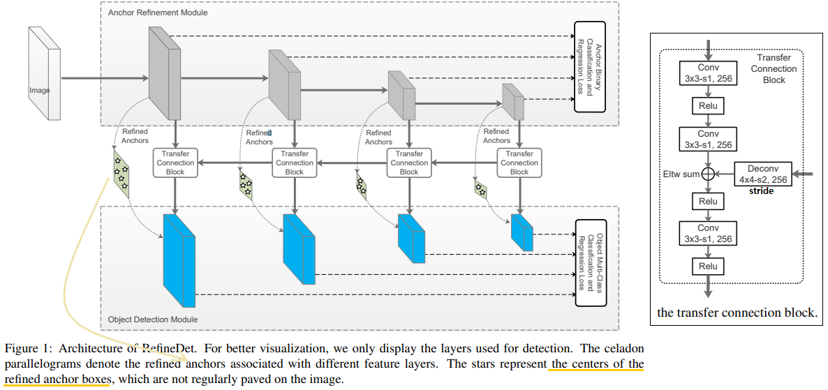
RefineDet은 SSD 계열의 모델이다. (아래 model Architecture 사진 참조)
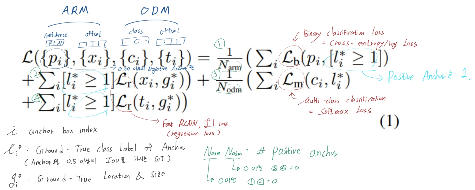
1) Anchor Refinement Module(ARM) : Anchor에 대한 binary classification수행. negative anchor들을 걸러내면서, 동시에 anchor들의 위치를 조절(RetinaNet에서 Focal Loss, YOLOv3에서 Objectness score 역할 for class imbalance)
2) Object Detection Module
RefineDet의 종류는 (input size) 320, 512, (with Multi-Scale Testing) + 가 있다.
최근 논문인 M2Det에서도 "Multi-Scale Testing기법"을 적극적으로 사용해 성능을 많이 올렸다. 특히 AP_small 에서 훨씬 좋은 성능을 얻어 내었다.
Multi-Scale Testing Algorithm
Filp과 UpScaling, DownScaling을 사용한다. 원본 이미지가 작을 수록 UpScaling을 많이 한다. 이 경우 Small Object 검출 성능을 높히고 FalsePositive(신경망은 객체라고 판단했지만 GT에는 아닐 경우)를 방지하기 위해 일정 크기 이하의 검출 결과만 사용한다.
모든 Scale에서 Inference한 결과를 모아서 NMS를 적용한다.
"""
im_detect(net, im, ratio*targe_size) : im를 ratio만큼 늘리거나 줄여서 inference 수행
마지막 모든 결과를 모아서 NMS 수행
"""det0=im_detect(net,im,targe_size)det0_f=flip_im_detect(net,im,targe_size)det1=im_detect(net,im,int(0.6*targe_size))det1_f=flip_im_detect(net,im,int(0.6*targe_size))det2=im_detect(net,im,int(1.2*targe_size))det2_f=flip_im_detect(net,im,int(1.2*targe_size))det3=im_detect(net,im,int(1.4*targe_size))det3_f=flip_im_detect(net,im,int(1.4*targe_size))det4=im_detect(net,im,int(1.6*targe_size))det4_f=flip_im_detect(net,im,int(1.6*targe_size))det5=im_detect(net,im,int(1.8*targe_size))det5_f=flip_im_detect(net,im,int(1.8*targe_size))cls_dets=np.row_stack((det0,det_r,det1,det2,det3,det4,det5,det7))cls_dets=soft_bbox_vote(cls_dets)# nms 적용
1-2 Paper Review
Conclusion
ARM (anchor refinement module)
negative anchors를 필터링 한다. classifier의 search sapce를 줄이기 위해서.
SSD -> DSSD (SSD+Deconvolution) -> DSOD(learn object detectors from ‘scratch’) -> Focal Loss, classification strategies(for class imbalance problem)
Network Architecture
핵심은 이와 같다,
TCB, ARM, ODM
Two-step cascaded regression
Negative anchor filtering
transfer connection block (TCB)
Eltw sum = sum them in the element-wise way
ARM으로 부터 내려오는 Feature는 the feature maps associated with anchors(Anchor에 대한 정보를 담고 있는 feature) 라고 할 수 있다.
Two-step cascaded regression
과거 모델들 단점 : the small objects 검출에 관한 낮은 성능
ARM에서 Anchors의 size와 location을 조정한다!
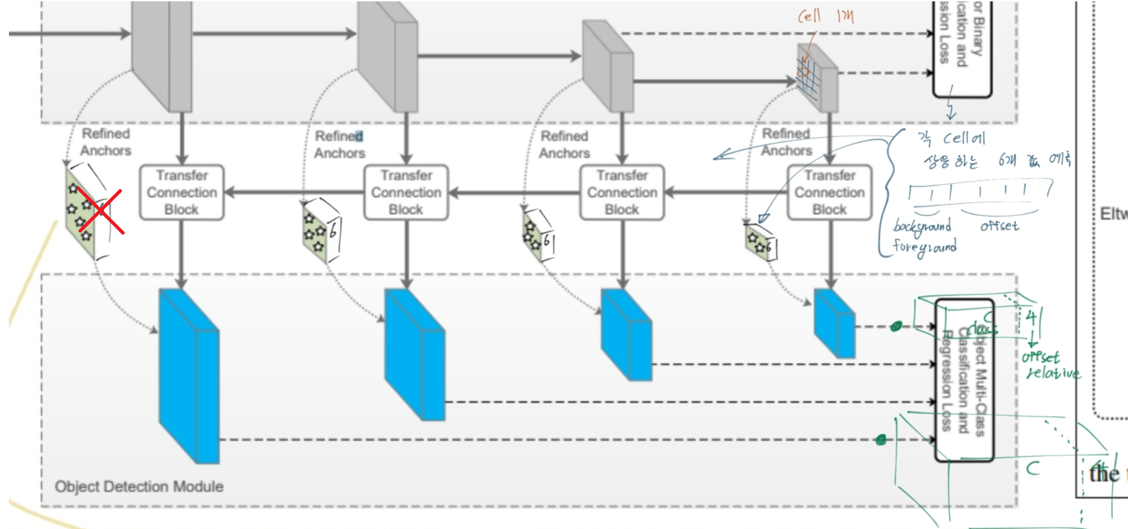
하나의 cell에 n개의 anchor box를 할당한다. 각 cell에 대해 4개의 offset값, 2개의 confidence score(background=negative, foreground=positive) 값을 예측한다. (총 6개 값이 ARM에서 예측됨 = the refined anchor boxes feature)
ODM에서는 각 cell에 대해서 c+4의 channel이 output으로 나오게 설정한다.
빨간색 X의 의미는 틀렸다는 의미다!! celadon parallelogram(청자색 평행사변형) 의 feature가 6 channel로 concat되는게 아니다. 코드를 확인해 보면 다음과 같이 설명할 수 있다.
“ARM에서 만들어지는 변수 arm_loc, arm_conf는 loss를 계산하는데 사용된다. 이 Loss값을 줄이기 위해 arm_loc, arm_conf는 최대한 정답값에 가까워지기 위해 노력한다. 그 말은 ARM의 Feature map(코드에서 Source변수)들이, arm_loc, arm_conf이 정확하게 나오도록, 값이 유도된다는 뜻이다. 이 과정을 통해 ARM의 Feature map은 ODM에서 Localization, Detection을 하기 위해 필요한, 충분한 정보를 담게 된다는 것을 의미한다.”
Negative Anchor Filtering
2개의 confidence score 중 negative 값이 일정 threshold(=0.99) 이상 보다 크면, ODM training 중에 사용하지 않는다. 이 과정에서 너무 많은 negative anchor가 제외되고, negative anchor box에 대한 loss값은 줄어든다. (Focal Loss 때의 Post 참조)
inferene 동안에 negative값이 너무 커도, ODM에서의 detection값은 무시된다.
Training and Inference
Anchors Design and Matching
stride : sizes 8, 16, 32, and 64 pixels
scale : stride x 4
ratios : three aspect ratios (i.e., 0.5, 1.0, and 2.0)
GT와 the best overlap score를 가지는 Anchor box를 matching 시킨 후, 그리고 0.5이상의 IOU를 가진 Anchor box를 매칭 시켰다. (?) (그렇다면 Positive, Negative 값의 GT값이 무엇인지 궁금하다. 코드를 봤지만 나중에 필요하면 다시 찾아보는게 좋겠다.)
Hard Negative Mining
대부분의 ARM_confidence값이 큰 Negative를 가진다. 너무큰 Negative를 가지는 값은 ODM에서 나오는 c+4값은 무시된다. (즉 Negative값이 Focal loss나 objectness score로 사용된다.)
training 에서 top loss를 만들어내는 Negative anchor에 대해서만 ODM 학습을 한다.(위의 설명처럼, 예측 negative값이 1에 가깝지 않을수록 negative anchor에 대한 loss가 커진다.) 거기다가 한술 더떠서 SSD의 hard Negative Mining기법을 사용해서, Negative : Positive의 비율을 3:1정도로 유지 되도록 anchor를 준비해 loss값을 계산한다.
Loss Function
ARM을 위한 Loss, ODM을 위한 Loss로 나뉜다.
여기서 궁금한것은 (1)번 항에서 Negative(=background)와 Positive(=foreround)에 대한 모든 학습이 이뤄질텐데, 왜 Positive anchor갯수만 사용하는 N_arm으로 나누지? 코드를 봐도 그렇다. 이유는 모르겠다. 하지만 큰 의미는 없는 듯 하다.
ARM에서 anchor를 refine하고 그거를 다시 ODM에서 anchor refine한 값이 예측 Bounding Box 좌표
Out으로 나오는 모~든 예측 Bounding box 중에서, confidence가 놓은 순서로 400개의 예측 box를 찾고, 그 400개에 대해서 NMS를 수행한다.
좀 더 정확한 사항은 ‘detection_refinedet.py-NMS수행’ 파일 참조. (논문에 이상하게 쓰여 있다)
Experiment
모든 데이터에 대해서, multi-scale testing 기법을 사용해서 더 좋은 결과를 얻었다. (블로그와 달리 이 논문에서는 multi-scale testing에 대한 설명은 하나도 없다. “그냥 썼다.”가 끝이다. 몇배를 어떻게 하고~ 에 대한 이야기는 없다. )
classRefineDet(nn.Module):"""
sources = list() : VGG를 통과하고 나오는 중간중간의 faeture map들
tcb_source = list() : Source에서 (ARM처리를 일단 하고) TCB처리를 하고 나오는 feature map
arm_loc = list()
arm_conf = list()
odm_loc = list()
odm_conf = list()
(A)1 내가 신기한것은 odm_loc를 계산한는데, arm_loc를 절대 사용하지 않는다. [(A)2,(A)3 이어서...]
"""def__init__(...):self.detect=Detect_RefineDet(num_classes,self.size,...)# arm, odm, tcb 구현에 필요한 layer 등록
defforward(self,x):# 84 ~ 103 Line : Sources 변수에 VGG Conv2D 통과+계산해서 값 넣기
# 106 ~ 129 Line : ARM처리하고 arm_loc, arm_conf 만들어 내고, tcb_source 변수에 값 넣기
# 131 ~ 149 Line : ODM처리하고 odm_loc, odm_conf 만들어 넣기
# 139 ~ ... Line : 아래와 같이 arm_loc, arm_conf, odm_loc, odm_conf 최종값 return 하기
ifself.phase=="test":output=self.detect(arm_loc.view(arm_loc.size(0),-1,4),# arm loc preds
self.softmax(arm_conf.view(arm_conf.size(0),-1,2)),# arm conf preds
odm_loc.view(odm_loc.size(0),-1,4),# odm loc preds
self.softmax(odm_conf.view(odm_conf.size(0),-1,self.num_classes)),# odm conf preds
self.priors.type(type(x.data))# default boxes
)# 정제된 값을 결과로 주세요! (최종 Bounding Box, What max conf class)
else:output=(arm_loc.view(arm_loc.size(0),-1,4),arm_conf.view(arm_conf.size(0),-1,2),odm_loc.view(odm_loc.size(0),-1,4),odm_conf.view(odm_conf.size(0),-1,self.num_classes),self.priors# anchor box의 가장 기본 위치 저장되어 있음
)returneoutput
classDetect_RefineDet(Function):"""
Decode predictions into bboxes.
test시에 나오는 결과 값은 c+4개 confidence, localization 값이 아니다.
이렇게 결과를 내보내면 사용자는 이게 뭔 값인지 절대 모른다.
따라서 max confidnence class값이 무엇인지, 최종 예측 bounding box가 무엇인지 정제해서 값을 던져주어야 한다. 이 클래스는 그런 역할을 한다.
(A)3 그러면서 Detect_RefineDet함수가 돌아갈때는 '기본 Anchor위치에 arm_loc를 먼저 적용하고, 그 다음에 odm_loc를 적용해서 나오는 예측 bounding box 값'을 정답값으로 사용한다.
"""foriinrange(num):default=decode(arm_loc_data[i],prior_data,self.variance)default=center_size(default)decoded_boxes=decode(loc_data[i],default,self.variance)
RefineDet.PyTorch/train_refinedet.py
deftrain():"""
(A)2 loss를 계산할 때, '기본 Anchor위치에 arm_loc를 먼저 적용하고, 그 다음에 odm_loc를 적용해서 나오는 예측 bounding box 값'을 가지고 loss를 계산하는 줄 알고 코드를 확인해 봤더니... 그것도 아니다. (내가 잘 못찾는 거일 수도 있다.)
"""refinedet_net=build_refinedet('train',cfg['min_dim'],cfg['num_classes'])arm_criterion=RefineDetMultiBoxLoss(2,0.5,True,...)odm_criterion=RefineDetMultiBoxLoss(cfg['num_classes'],0.5,True,...)net=refinedet_netout=net(images)optimizer.zero_grad()# RefineDetMultiBoxLoss 가 정의된 refinedet_multibox_loss.py 파일을 보면 (A)2 결론을 내릴 수 있다.
arm_loss_l,arm_loss_c=arm_criterion(out,targets)odm_loss_l,odm_loss_c=odm_criterion(out,targets)arm_loss=arm_loss_l+arm_loss_codm_loss=odm_loss_l+odm_loss_closs=arm_loss+odm_lossloss.backward()
# 구체적으로 설명할 수 없지만, 궁금한게 Loss함수에 많이 구현되어 있다. 자주 볼거다.
defaults=priors.data# Anchor들이 '이미지 위'에 위치하는 위치()를 정확하게 적어놓은 값.
ifself.use_ARM:refine_match(self.threshold,truths,defaults,self.variance,labels,loc_t,conf_t,idx,arm_loc_data[idx].data)else:refine_match(self.threshold,truths,defaults,self.variance,labels,loc_t,conf_t,idx)
RefineDet.PyTorch/layers/box_utils.py
defrefine_match(threshold,truths,priors,variances,...):"""
(A)4 내가 (A)2에서 했던 말이 맞았다!!
loss를 계산할 때, refine_match라는 함수를 통해서 만약 ODM에 대한 odm_loc_data를 계산하고 싶다면, priors 위치를 한번 arm_loc_data로 offset refine한 후, 다시 odm_loc_data로 offset refine하고 나서 원래 GT-bounding box 위치랑 비교를 한다.
이 함수에서 그러한 작업을 수행한다.
"""
겨우 5페이지 밖에 안되는 논문이기 때문에, 궁금한것만 대충 읽고 Youtube의 발표 자료를 이용해 공부하려고 한다. 또한 모르는 것은 코드 중심으로 공부해야겠다. 그럼에도 불구하고, 역시 내가 직접 논문을 읽는게 직성이 풀린다. 그리고 누군가의 설명을 들으면 솔직히 의심된다. 이게 맞아? 그리고 정확히 이해도 안된다. 물론, 논문도 자세하지 않기 때문에 누군가의 설명을 참고해서 직관적인 이해를 하는 것도 좋지만, Yolov3는 논문이 신기한 논문이라서, 논문 그 자체로도 이해가 잘 됐다.
Anchor(=bounding box != GT_object)를 이용한 the relative offset 개념을 그대로 사용한다.
이전 모델들과 다르게, 각 bounding-box가 an objectness score 개념을 사용한다. 한 객체에 대해서 가장 많이 겹친 box만 objectness score target = 1을 준다. (지금까지 IOU (+confidence)를 이용해서 일정 이상의 값이면 Positive라고 판별하고 objectness score = confidence = 1 을 주었다.)
only assigns one bounding box prior for each ground truth object
한 객체 GT에 대한 하나의 bounding box 이외에, 다른 박스들은 class predictions와 coordinate(offset)으로 어떤 loss도 발생시키지 않는다. 단지 objectness sore에 의한 loss만 적용된다.
Class Prediction
not use a softmax for multilabel classification. Yes logistic classifiers
binary cross-entropy loss
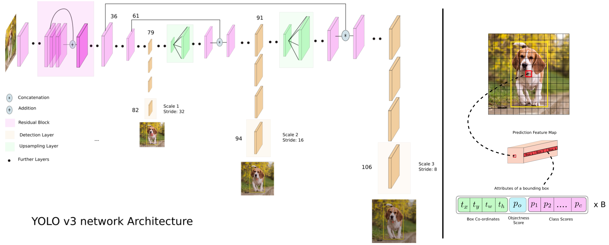
Predictions Across Scales
주황색 단이 우리가 SSD나 RetinaNet에서 보는 detect-head classification, regression 단이다.
위와 같이 3개의 P(pyramid feature)를 사용한다. 그리고 하나의 cell에 대해서, 3개의 Anchor box만 사용한다.
COCO dataset에 대해서, K-mean clustering을 사용해서 가장 적절한 bounding box(Anchor box 크기)값을 찾는다. 결론적으로 (10×13),(16×30),(33×23) // (30×61),(62×45),(59× 119) // (116 × 90),(156 × 198),(373 × 326) 를 사용한다. (동영상 : 내가 찾고자 하는 객체의 특징을 반영해서 bounding box크기를 적절히 설정하는 것도 아주 중요하다. 예를 들어 사람을 detect하고 싶다면 가로로 긴 박스는 필요없다)
당연히 작은 bounding box는 가장 마지막 단의 cell에서 사용되는 box, 큰 bounding box는 가장 첫번째 단의 cell에서 사용되는 box이다.
Things We Tried That Didn’t Work
Offset predictions : linear 함수를 사용해봤지만 성능 저하.
Focal Loss : objectness score라는 개념이 들어가서, 이것으로 easy, hard Image에 따른 성능 저하는 없었다. 차라리 Focal Loss를 사용해서 성능 저하가 일어났다. 또한 objectness score 덕분에 hard negative mining과 같은 작업을 하지 않았다. 즉 objectness score를 통해 class imbalance 문제를 다소 해결했다.
Dual IOU thresholds and truth assignment : Faster RCNN 에서는 2개의 IOU thresholds를 사용했다. (0.7과 0.3) 0.7을 넘으면 Positive example, 0.7과 0.3 사이는 학습에 사용하지 않고, 0.3 이하는 Negative example로 background 예측에 사용했다. 비슷한 전력을 사용했지만 결과는 좋지 않았다.
COCO의 AP 계산에 대한 비판
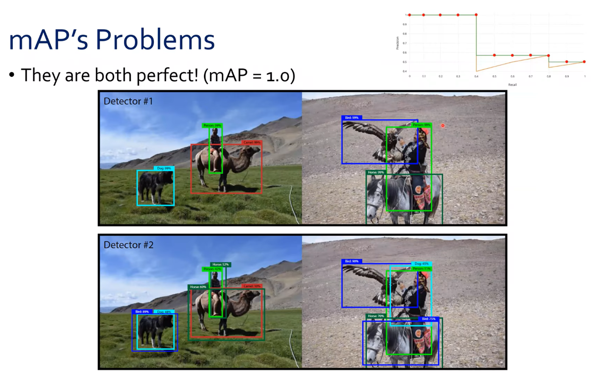
YOLOv3는 좋은 detector이다. 하지만 COCO AP는 IOU를 [0.5부터 : 0.95까지 : 0.05단위로] 바꾸며 mAP를 계산한다. 이건 의미가 없다! 인간이 IOU 0.3~0.5를 눈으로 계산해보라고 하면 못하더라!
COCO에서는 Pascal voc보다 labelling 이 정확한건 알겠다.(Bounding Box를 정확하게 친다는 등) 하지만 IOU가 0.5보다 정확하게 Detect해야한다는 사실은 의미가 없다. 0.5보다 높게 Threshold를 가져가면… classification은 정확하게 됐는데, regression 좀 부정확하게 쳤다고 그걸 틀린 판단이라고 확정해버리는 것은 억울하다.
mAP는 옳지 않은 지표이다.
이 그림에서 위의 Detector 1 이 훨씬 잘했다고 우리는 생각한다. 하지만 둘다 mAP를 계산하면 놀랍게도 1이 나온다. 2개를 이용해 recall, precise 그래프를 그려보면 오른쪽 위와 같은 그래프가 된다. 초록색 라인이 Detector1이고 주황색 라인이 Detector2이다!
docker run -d\-p 8080:8080 \ # port 설정 --name"ml-workspace"\-v"${PWD}:/workspace"\--envAUTHENTICATE_VIA_JUPYTER="mytoken"\--shm-size 512m \--restart always \
mltooling/ml-workspace:0.12.1
ctrl+shift+p -> Remote-Containers: Open Attached Container Configuration File
5. detectron2 using ml-workspce
import torch, torchvision
print(torch.__version__, torch.cuda.is_available())
import detectron2
from detectron2.utils.logger import setup_logger
setup_logger()# import some common libraries
import numpy as np
import os, json, cv2, random
# import some common detectron2 utilities
from detectron2 import model_zoo
from detectron2.engine import DefaultPredictor
from detectron2.config import get_cfg
from detectron2.utils.visualizer import Visualizer
from detectron2.data import MetadataCatalog, DatasetCatalog
im = cv2.imread("./input.jpg")
cfg = get_cfg()
cfg.merge_from_file(model_zoo.get_config_file("COCO-InstanceSegmentation/mask_rcnn_R_50_FPN_3x.yaml"))
cfg.MODEL.ROI_HEADS.SCORE_THRESH_TEST = 0.5 # set threshold for this model
cfg.MODEL.DEVICE ="cpu"# 필수!!!!
cfg.MODEL.WEIGHTS = model_zoo.get_checkpoint_url("COCO-InstanceSegmentation/mask_rcnn_R_50_FPN_3x.yaml")
predictor = DefaultPredictor(cfg)
outputs = predictor(im)
print(outputs["instances"].pred_classes)
print(outputs["instances"].pred_boxes)
디버깅이 안된다. Step into로 들어가면, 내가 보고 있는 py파일 뿐만 아니라, Import하는 함수 내부로 들어가서 어떤 파일과 함수가 실행되는지 보고 싶은데 안된다. docker container 내부, ubuntu의 env 속, python 모듈은 디버깅으로 들어갈 수 없는 건가??
에러내용 - DefaultPredictor가 어떤 흐름으로 실행되는지 대충 훔처 볼 수 있다.
AssertionError:
Torch not compiled with CUDA enabled
# /opt/conda/bin/python /workspace/test.py
1.7.1 False
** fvcore version of PathManager will be deprecated soon. **** Please migrate to the version in iopath repo. **
https://github.com/facebookresearch/iopath
** fvcore version of PathManager will be deprecated soon. **** Please migrate to the version in iopath repo. **
https://github.com/facebookresearch/iopath
model_final_f10217.pkl: 178MB [01:03, 2.79MB/s]
# MODEL.DEVICE = 'cpu' -------------------------------------------------------------------------------------------------------------------------------------------------------------------------------------------------------
test.py 29 <module>
outputs = predictor(im)
defaults.py 223 __call__
predictions = self.model([inputs])[0]
module.py 727 _call_impl
result = self.forward(*input, **kwargs)
rcnn.py 149 forward
return self.inference(batched_inputs)
rcnn.py 202 inference
proposals, _ = self.proposal_generator(images, features, None)
module.py 727 _call_impl
result = self.forward(*input, **kwargs)
rpn.py 448 forward
proposals = self.predict_proposals(
rpn.py 474 predict_proposals
return find_top_rpn_proposals(
proposal_utils.py 104 find_top_rpn_proposals
keep = batched_nms(boxes.tensor, scores_per_img, lvl, nms_thresh)
nms.py 21 batched_nms
return box_ops.batched_nms(boxes.float(), scores, idxs, iou_threshold)
_trace.py 1100 wrapper
return fn(*args, **kwargs)
boxes.py 88 batched_nms
keep = nms(boxes_for_nms, scores, iou_threshold)
boxes.py 41 nms
_assert_has_ops()
extension.py 62 _assert_has_ops
raise RuntimeError(
RuntimeError:
Couldn't load custom C++ ops. This can happen if your PyTorch and torchvision versions are incompatible, or if you had errors while compiling torchvision from source. For further information on the compatible versions, check https://github.com/pytorch/vision#installation for the compatibility matrix. Please check your PyTorch version with torch.__version__ and your torchvision version with torchvision.__version__ and verify if they are compatible, and if not please reinstall torchvision so that it matches your PyTorch install.
6. Debug Docker Containers
명학이의 도움으로 다음의 과정을 진행해 보았다. -> 안됨
ctrl + shift + p -> setting -> > debug : launch json 검색-> Python file 선택
$ docker run -d\-p 8080:8080 \ # port 설정 --name"ml-workspace"\-v"${PWD}:/workspace"\--envAUTHENTICATE_VIA_JUPYTER="mytoken"\--shm-size 512m \--restart always \--entrypoint=bash
mltooling/ml-workspace:0.12.1
$ docker exec-it <docker-container-name or ID> bash
# new shell start $ python
>> 여기서 module 디버깅
우분투에서 ctrl + shift + p -> > debug : launch json 검색-> Python file 선택 이 파일 내부의 내용을 아래 처럼 수정한다.
사실 아래처럼 다 바꿀 필요는 없고, 진짜 중요한 것은 justMyCode : false 이다. 이것만 처리해주면 된다.
{
     // Use IntelliSense to learn about possible attributes.
     // Hover to view descriptions of existing attributes.
     // For more information, visit: https://go.microsoft.com/fwlink/?linkid=830387
     "version": "0.2.0",
     "configurations": [
         {
             "name": "Python: Current File",
             "type": "python",
             "request": "launch",
             "program": "${file}",
             "console": "integratedTerminal",
             "debugOptions" : ["DebugStdLib"],
             "justMyCode": false
           }
     ]
 }
하지만!! SSH server’s Docker container에서는 debug json 검색해도 찾을 수가 없었다. 더 쉬운 다른 방법은 이것을 클릭하면 된다!
{//UseIntelliSensetolearnaboutpossibleattributes.//Hovertoviewdescriptionsofexistingattributes.//Formoreinformation,visit:https://go.microsoft.com/fwlink/?linkid=830387"version":"0.2.0","configurations":[{"name":"Python: Current File","type":"python","request":"launch","program":"${file}","console":"integratedTerminal","debugOptions":["DebugStdLib"],"justMyCode":false}]}
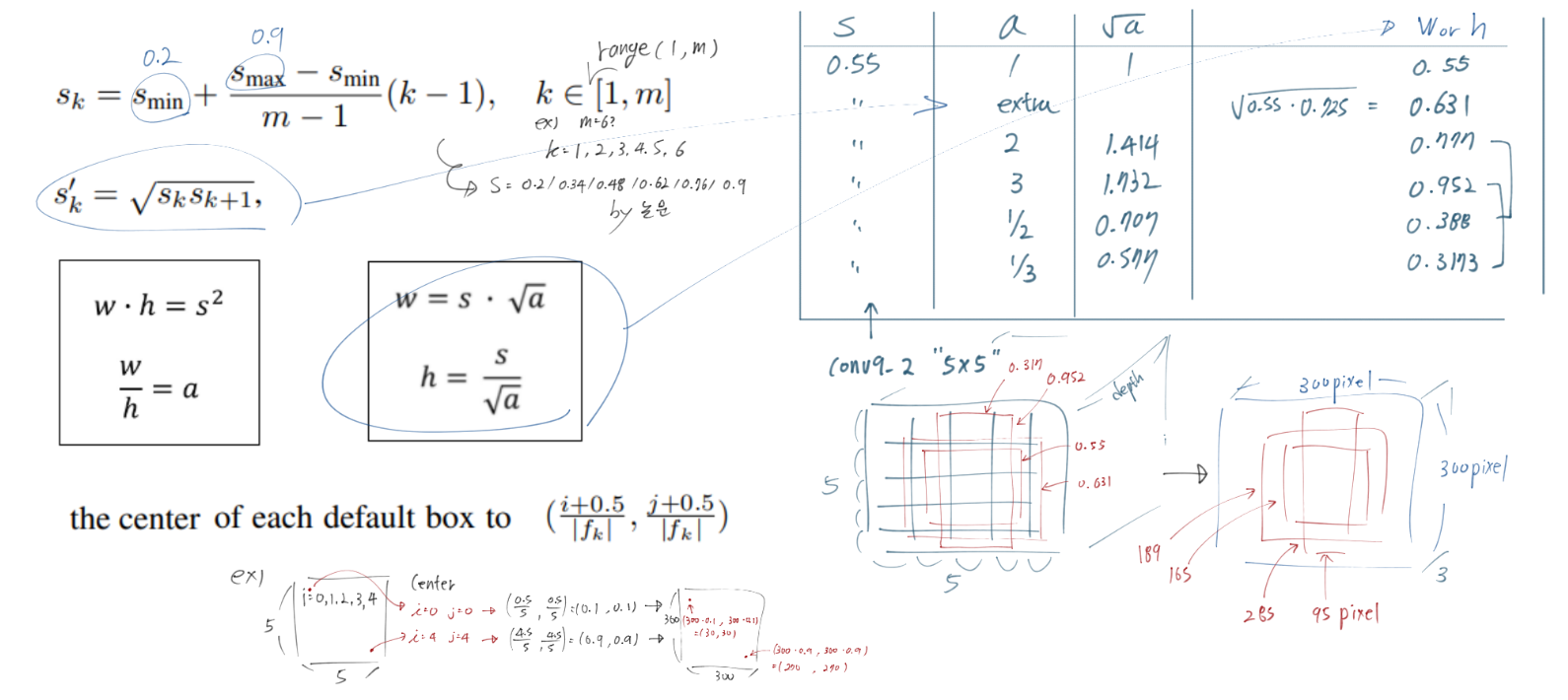
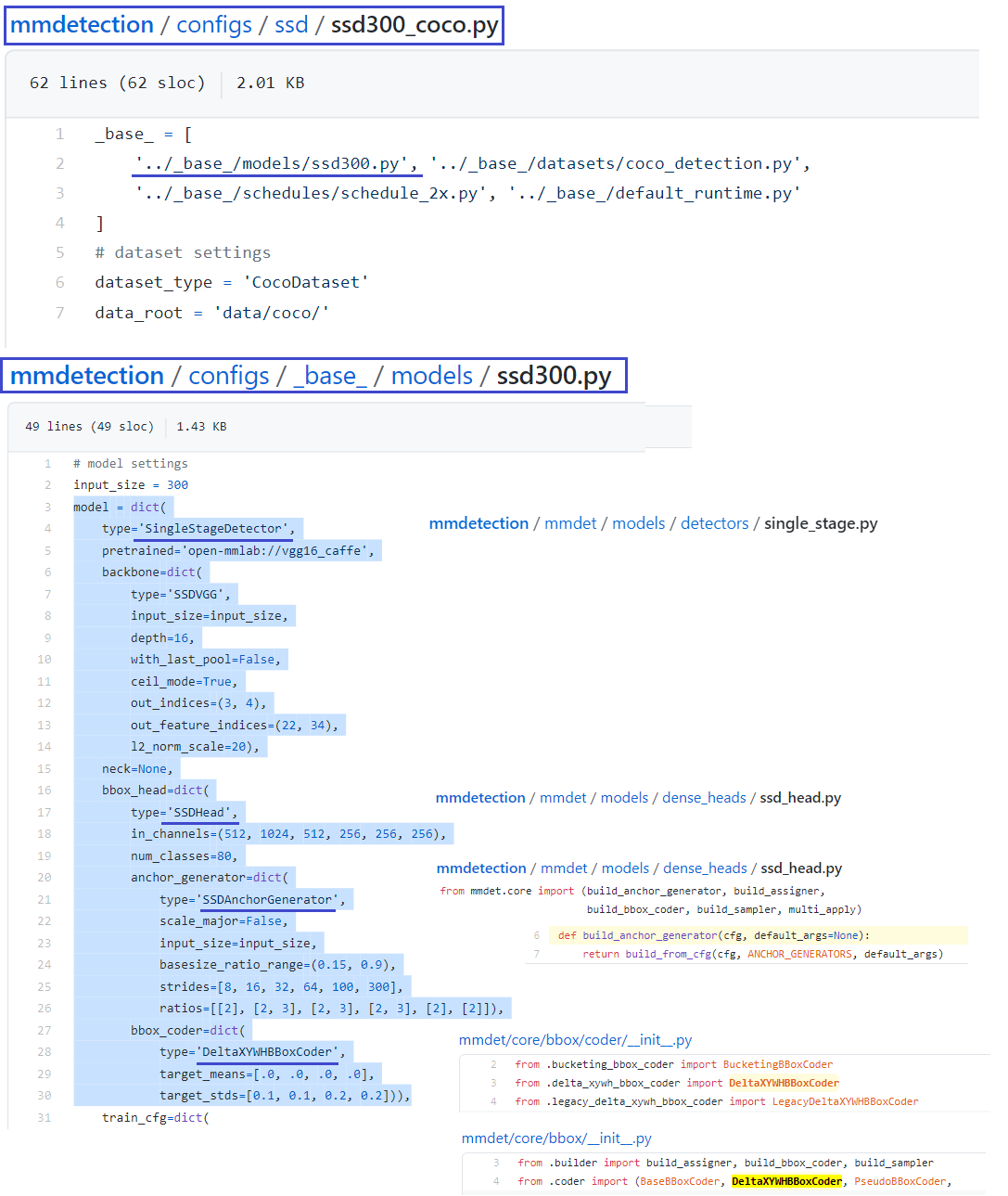
이번에 참고한 코드가 너무 쉽게 잘 되어 있어서 맘에 든다. SSD에서는 Anchor생성을 위해 s라는 개념을 사용했는데, 이 코드와 논문에서는 s의 개념을 사용하지 않는다.
그래서 이 anchor 사이즈가 적당한거야? 라는 생각이 들긴 한다. 이 정도 anchor사이즈면 이미지에 어느정도 크기로 (anchor box를) 대보는거지? 라는 생각이 들지만 굳이 그런 수학적 계산을 할 시간은 없다.
역시 논문만 봐서는 자세하게 이해못하는게 당연하다. 코드를 봐야 이해가 된다.
1. RetinaNet
Abstract, Introduction, Related Work
Class Imbalance :
one-stage detector는 너무 많은 candidate location을 추론한다.(Faster-RCNN에서는 RPN에서 한번 거리고, 마지막 regression에서 한번 거리즈만..) 하지만 극히 일부만 진짜 object가 들어 있다. 이 이유는 2가지 이다.
(1) most locations are easy negatives(backgorund 혹은 크고 선병한 객체)-학습에 도움 안됨 (2) the easy negatives가 학습을 압도한다.
Class Imbalance문제를 focal loss를 사용해서 naturally, handle 하고 자 한다.
robust loss 라는 방식은 hard example의 loss를 더욱 키우는 방식이지만, focal loss에서는 반대이다. easy example의 loss를 아주 작게 만든다.
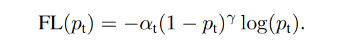
Focal Loss
γ는 2~5값을 사용했고, α는 balanced variable 이다. Focal loss의 정확한 형태(정확한 하이퍼파라메터값)은 중요하지 않다. 적당한 어떤 값이하도 효율적으로 작동한다.
for γ = 2, α = 0.25 works best
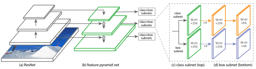
RetinaNet Detector
이 논문의 핵심은 Forcal Loss. to eliminates the accuracy gap between easy and hard examples. 따라서 Architecture는 아주 simple.
(c) subnet에 들어갈 Channels = 256 and # Anchor = 9. 그리고 Ryramid간의 parameter share는 안한다.
Anchors
On pyramid levels P3 to P7, areas of 32^2 to 512^2 개의 cell에 각각 Anchor가 적용된다.
classFocalLoss(nn.Module):defforward(self,classifications,regressions,anchors,annotations):# predict한 classifications, regressions 결과가 parameter로 들어온다.
# annotation에 Ground True값이 들어온다.
alpha=0.25gamma=2.0classification_losses=[]regression_losses=[]# 나중에 이 loss를 모아서 return
# 1. compute the loss - 이미지에 객체가 하나도 없을 때
# 2. compute the loss for classification
focal_weight=alpha_factor*torch.pow(focal_weight,gamma)bce=-(targets*torch.log(classification)+(1.0-targets)*torch.log(1.0-classification))# object, background 모두. targets =[1,0]
cls_loss=focal_weight*bce# 3. compute the loss for regression
""" L127 ~ L160까지 Anchor box와 GT와의 regression 계산 과정(SSDw/codePost 참조)= target"""regression_diff=torch.abs(targets-regression[positive_indices,:])regression_loss=torch.where(torch.le(regression_diff,1.0/9.0),0.5*9.0*torch.pow(regression_diff,2),regression_diff-0.5/9.0)returntorch.stack(classification_losses).mean(dim=0,keepdim=True),torch.stack(regression_losses).mean(dim=0,keepdim=True)
pytest는 패키지를 완성하는 동안, 하나의 .py파일을 test하는 하나의 좋은 모듈이다.
pytest이전에는 assert 기반의 unittest (wiki-unitest)가 많이 사용되었지만, 최근에 와서는 pytest가 더 편리해서, 더 많이 사용되는 듯 하다. (pypi에서 검색을 해봐도, unittest는 최근 update가 2015이고, pytest는 2021년이다. 또한 raddit에서도 ‘just use pytest’라고 한다.)
이 Pytest에 대해 공부해보자.
그럼에도 불구하고, detectron2와 mmdetection에서는 unittest를 사용한다. 하지만 연구실 석박사 선배님들이 Unit Test 모듈을 사용하시는 것 같지는 않다. 필요하면 그 때 찾아서 공부해, 보도록 하자.
Unit Test 란? 유닛이란 보통 함수 단위라고 생각하면 좀 더 이해가 될 겁니다. 프로그램은 결국 데이터와 이를 처리하는 함수로 구성되는데 각 함수를 충분히 테스트하면 전체 프로그램에서 문제가 발생하는 것을 최소화할 수 있을겁니다. 그래서 함수를 구현한 후 함수의 입력과 예상되는 출력을 비교함으로써 함수를 테스트하는 겁니다.
이 글을 통해서, Pytest는 디버깅을 하면서, 각 변수에는 어떤 type size(view) length 를 가지는지 확인하는 방법이 아니다. 라는 것을 깨달았다. 코드 내부에 구현한 함수 or 클래스가 잘 통작하는지? 어떤 인풋에 대해서 내가 원하는 Output이 나온지? 확인하는 모듈인 것 같다.
bounding box 내부의 객체 class에 상관없이, Box 내부에 masking 정보만 따내는 역할을 하는 Mask-branch를 추가했다.
Equivariance 연산(<-> Invariant)을 수행하는 Mask-Branch는 어떻게 생겼지? Mask-branch에 가장 마지막 단에 나오는 feature map은 (ROI Align이후 크기가 w,h라 한다면..) 2 x w * 2 x h * 80 이다. 여기서 80은 coco의 class별 mask 모든 예측값이다. 80개의 depth에서 loss계산은, box의 class에 대상하는 한 channel feature만을 이용한다. 나머지는 loss 계산시 무시됨.
ROI Align 이란? : Input-EachROI. output-7x7(nxn) Pooled Feature. nxn등분(첫번째 quantization)->각4등분(두번째 quantization)->Bilinear interpolation->각4등분에 대해 Max Pooling->(nxn) Pooled Feature Map 획득.
detectron2/modeling/meta_arch/build.py : def build_model(cfg): model = META_ARCH_REGISTRY.get(meta_arch)(cfg)
cfg.MODEL.META_ARCHITECTURE 에 적혀있는 model architecture 를 build한다. ( weight는 load하지 않은 상태이다. DfaultPredictor에서 model weight load 해준다. checkpointer.load(cfg.MODEL.WEIGHTS) )
from detectron2.utils.registry import Registry -> META_ARCH_REGISTRY = Registry("META_ARCH")
detectron2/utils/registry.py : from fvcore.common.registry import Registry
fvcore로 넘어가는거 보니… 이렇게 타고 가는게 의미가 없는 듯 하다.
따라서 다음과 같은 디버깅을 수행해 보았다.
model의 핵심은 GeneralizedRCNN 인듯하다. 따라서 다음의 파일을 분석해보기로 하였다.
detectron2/modeling/meta_arch/rcnn.py : class GeneralizedRCNN(nn.Module):
이 과정은 다음을 수행한다
Per-image feature extraction (aka backbone)
Region proposal generation
Per-region feature extraction and prediction
여기까지 결론 :
내가 원하는 것은, 원래 이해가 안됐다가 이해가 된 부분의 코드를 확인해 보는 것 이었다.(3.2 참조) 하지만 이 같은 코드 구조로 공부를 하는 것은 큰 의미가 없을 듯 하다.
어쨋든 핵심은 detectron2/detectron2/modeling 내부에 있는 코드들이다. 코드 제목을 보고 정말 필요한 내용의 코드만 조금씩 읽고 이해해보는게 좋겠다. 여기있는 클래스와 함수를, 다른 사용자가 ‘모듈로써’ 가져와서 사용하기 쉽게 만들어 놓았을 것이다. 따라서 필요하면 그때 가져와서 사용해보자.
코드가 모듈화가 거의 안되어 있다. model.py에 거의 모든 구현이 다 되어 있다. 그래서 더 이해하기 쉽다.
아래의 내용들이 코드로 어떻게 구현되었는지 궁금하다.
(1) RPN-Anchor사용법
(2) ROI-Align
(3) Mask-Branch
(4) Loss_mask
(5) RPN의 output값이 Head부분의 classification/localization에서 어떻게 쓰이는지
원래는 공부하려고 했으나… 나중에 필요하면 다시 와서 공부하도록 하자.
2020.02.04 - RefineDet까지 공부하면서 코드를 통해서 헷갈리는 것을 분명히 파악하는 것이 얼마나 중요한 것인지 깨달았다. 따라서 그나마 가장 궁금했던 것 하나만 빠르게 분석하려고 한다.
(5) RPN의 output값이 Head부분의 classification/localization에서 어떻게 쓰이는가?
RPN에서 나오는 2(positive, negative objectness score)+4(offset relative) = 6개의 정보.
위에서 나온 ROI 중에서, 정말 객체가 있을 법한 정제된 ROI 즉 rpn_rois를 추출
rpn_rois에서 4(offset relative) 값만 이용한다. Backbone에서 나온 Feature Map에서 저 4(offset relative)에 대한 영역만 ROI Pooing (ROI Align)을 수행한다.
**pytorch-mask-rcnn/model.py ** 코드로 확인
# pytorch-mask-rcnn/model.py
defproposal_layer(inputs,proposal_count,nms_threshold,anchors,config=None):"""
RPN에서 나온 결과들 중 정말 필요한 ROI만을 걸러주는 Layer
아래의 (bg prob, fg prob) = (negative=easy confidence, pasitive=hard confidence)를 이용해서 적당한
Inputs:
rpn_probs: [batch, anchors, (bg prob, fg prob)]
rpn_bbox: [batch, anchors, (dy, dx, log(dh), log(dw))]
Returns:
Proposals in normalized coordinates [batch, rois, (y1, x1, y2, x2)]
"""outputs=list(zip(*layer_outputs))# BackBone + RPN을 통과하고 나온느 결과들
outputs=[torch.cat(list(o),dim=1)foroinoutputs]rpn_class_logits,rpn_class,rpn_bbox=outputs# rpn_rois 위의 함수에 의해 나온 정제된 rpn_rois
rpn_rois=proposal_layer([rpn_class,rpn_bbox],proposal_count=proposal_count,nms_threshold=self.config.RPN_NMS_THRESHOLD,anchors=self.anchors,config=self.config)# rpn_rois가 self.classifier에 들어가는 것에 집중
ifmode=='inference':mrcnn_class_logits,mrcnn_class,mrcnn_bbox=self.classifier(mrcnn_feature_maps,rpn_rois)# rpn_rois가 detection_target_layer함수에 의해 rois가 되고, self.classifier에 들어가는 것에 집중
elifmode=='training':rois,target_class_ids,target_deltas,target_mask=detection_target_layer(rpn_rois,gt_class_ids,gt_boxes,gt_masks,self.config)mrcnn_class_logits,mrcnn_class,mrcnn_bbox=self.classifier(mrcnn_feature_maps,rois)
# self.Classifier가 무엇인가?
self.classifier=Classifier(256,config.POOL_SIZE,config.IMAGE_SHAPE,config.NUM_CLASSES)# Line 908
classClassifier(nn.Module):defforward(self,x,rois):# x : backbone 통과하고 나온 feature map
x=pyramid_roi_align([rois]+x,self.pool_size,self.image_shape# ** [rois]+x 에 집중!! list에 append 되는 거다! **
# 그 이후 conv2 계속 통과...
defpyramid_roi_align(inputs,pool_size,image_shape):"""
feature map을 받고 거기서 ROI Pooing => ROP Align 을 수행해 reture해주는 함수
Inputs = [rois]+x
Input[0] : refined boxes by 'proposal_layer' func - [batch, num_boxes, (y1, x1, y2, x2)
Input[1] : Feature maps - List of feature maps from different levels
Input[0] 가 가리키는 영역에 대해서 Input[1]에서 부터 ROI Aling(Pooing)을 수행한다.
return [pooled feature map : RPN이 알려준, Feature Map 중에서 '객체가 있을법한 영역'만 뽑아낸 조각난 Feature map]
"""
저자 : Wei Liu , Dragomir Anguelov, Dumitru Erhan , Christian Szegedy
읽는 배경 : Recognition Basic. Understand confusing and ambiguous things.
읽으면서 생각할 포인트 : 이전 나의 SSD 정리 Post, 코드와 함께 최대한 완벽히 이해하기. 이해한 것 정확히 기록해두기.
느낀점 :
논문을 정말 깔끔하게 정리해놓은 사이트(SSD 분석)이 있다. 내용도 좋지만, 어떻게 논문을 정리 했는지를 참고하자. 지금은 논문을 추후에 작성하기 위해, 내용을 아주 짧게 요악하는 것 보다는 논문의 논리전개가 어떤지 기록하고 있다. 하지만 어느정도 익숙해지면, 이와 같은 논문 정리가 필요한 것 같다. 정말 핵심적인 내용만! 사실 논문이 말하는 ‘핵심’은 한 문단으로도 충분히 설명 가능하다. 그것만 기억해 두면 된다는 사실을 잊지 말자.
하지만 내가 위의 사이트를 참고하지 않는 이유는, 저런 논문 정리는 이미 많이 봤다. 내가 직접 논문을 읽고 도대체!! Bounding Box를 어떻게 사용하고, Loss함수를 어떻게 정의해서 사용하는지. 내가 직접 논문 읽고 이해하고 싶었기 때문이다.
SSD논문 자체도 그리 자세하지 않다… 원래 논문이 이렇게 자세하지 않을 수 있나보다. 만약 논문을 읽으면서 완벽하게 이해되지 않았다면, (1) 논문에는 잘 적혀있는데 내가 이해하지 못했거나 (2) 논문이 원래 자세하지 않거나. 둘 중 하나이다. 따라서 논문을 읽고 100프로 이해가 안됐다고 해도, (2)경우일 수 있으니, 모른다고 좌절하지 말자.
선배 조언
날 먼저 판단하지 마라. 박사나 석사나 학사나 똑같다. 동급이다. 누가 더 잘하고 못하고가 없다. 내가 궁금한 분야를 좀만 공부하면, 금방 그 이상의 실력을 가질 수 있다.
자신있게 하고 싶은걸 해라.
느낀점 :
카이스트는 주중과 주말 상관없이 모든 사람이 열심히 공부하고 연구하고 그러는 줄 알았다. 하지만 내가 상상한 그 정도는 아니었다. 여기 계신 분들도 토일 쉬고 점심,저녁 2시간씩 쉬고 쉬고 싶은날 쉬고 그러시는 것 같다. (물론 집에서도 조금씩 공부하시지만..) 그러면 여기 계신 분들이 우리나라에서 많은 좋은 결과,논문들을 만들어 내는 이유가 뭘까? 생각해보았다. 그냥 맘먹으면 무언가를 해낼 수 있는 사람들이 모여있기 때문인 것 같다.(즉, 좋은 사람들이 함께 모여있기 때문.) 여기에 좋은 사람들이 너무 많다. 내가 노력하면 정말 좋은 conference의 논문에 2저자 3저자로 내가 들어갈 수 있게 해줄 똑똑한 사람들, 착한 사람들, 그리고 뭔가를 독하게 해본 사람들, 좋은 조언을 해줄 수 있는 사람들이 아주 많다. 이런 분들이 많이 보여 있기 때문에 나같은 후배들이 더 빠르게 위로 올라올 수 있는 것 같고, 그렇게 빠르게 올라온 사람들은 다음에 올 아래의 사람들(후배)들을 똑같이 빠르게 끌어올려 줄 수 있는 것 같다. 이런 ‘선 순환’으로 대한민국 최고의 대학이 될 수 있지 않았나 싶다. 절대적인 공부시간은 다른 대학의 사람들과 똑같다 할지라도.
따라서. 나도 할 수 있다. 여기 계신 분들이 주말에는 푹 쉬고 점심저녁에 좀 놀고 가끔은 노는 시간에..! 나는 공부하고 공부하고 노력하면, 나도 충분히 여기 계신 분들처럼 좋은 결과를 내고, 좋은 논문을 낼 수 있겠다는 자신감이 생긴다. 지금은 여기 계신 분들보다 지식은 많이 부족해도. 여기 계신 그 어떤 분보다, 노력이 부족한 사람은 되지 말자. 따라잡고 싶으면, 보다 더 해야지. 닮고 싶다면, 더 일찍 더 늦게까지 공부해야지. 당연한거다.
1. Single Shot Detector - SSD
Abstract, Introduction
SSD
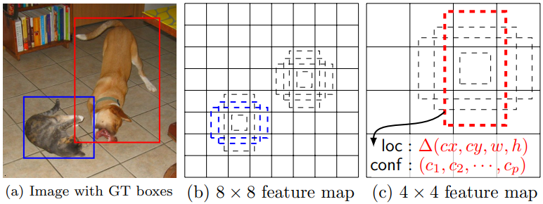
each default box를 통해서 예측하는 2가지. (1) the shape offsets relative and (2) the confidences
In Traning, Default Box와 GT Box를 matching값을 비교한다. 아래의 사진의 빨간색, 파란색 점선처럼 Positive인 것만을 다른다. 나머지는 Negative. 이다. 이때 사용하는 Loss함수는, localization loss (e.g. Smooth L1) and confidence loss (e.g. Softmax)
Positive에 대해서는 Confidence & regressing Loss를 모두 학습시키고, Negative에 대해서는 Confidence에 대해서만 학습 시킨다.
Predictions of detections at multiple scale object.
m × n with p channels의 feature map -> 3 × 3 × p small kernel -> m × n x (class confidence score + shape offset relative(GT에 대한 Default box의 상대적 offset값)) = [(c + 4)*k] channels
Training
Matching strategy : IOU가 0.5 이상인 것만을 Positive로 사용했다. (그 이외 자세한 내용 없음)
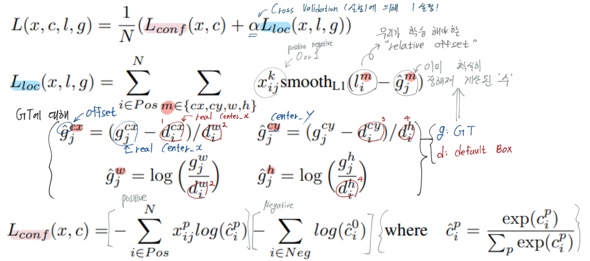
Loss 함수 이해하기
N : positive dafault box 갯수 = the number of matched default boxes
N이 0이면 loss는 0이다. (최저 Loss값 따라서 학습 이뤄지지 않음)
k : category
x : i번재 default box, j번째 GT box에 대한 매칭 값 {1 positive,0 negativ}
l : the predicted offset relative
g : the ground truth box
d : the default bounding box
localization : For the center (cx, cy) and r its width (w) and height (h)
sharing parameters across all object scales (가장 마지막 단의 classification, localization에 대해)
이번에 다시 보는 이유는, SSD paper를 읽고, SSD에서 이해가 안됐던 내용을 코드를 통해 공부하고, 혹은 이 논문 부분을 코드로 어떻게 구현했지? 를 알아보기 위해 공부한 내용을 정리하기 위함이다.
원래 이해가 안됐다가, 이해가 된 [(1)Localization Loss function 이해하기] [(2)default boxes about scales and aspect ratios] 는 코드에서 정확히 어떻게 구현되어 있는지 공부해 보자.
이라고 생각했으나, RetinaNet의 코드가 너무 깔끔하고 이쁘다.(물론 모듈화는 SSD이 코드가 더 잘되어 있지만.. 모듈화가 많이 되었다고 좋은 건 아닌 듯 하다. 코드를 처음 보는 사람이 머리 아프다.) 위의 (1)(2) 또한RetinaNet 코드로 대강 알 수 있기 때문에 그것을 보는게 더 좋을 듯 하다.
2021-02-04 : SSD 코드를 공부했을때 모듈화가 심각해서 보기가 힘들었다. 하지만 그것은 “처음부터 끝까지 다 봐야지.” 라는 욕심때문에 보기 힘들었던 것 같다. 하지만 사실 그렇게 코드를 보는 경우는 드믄것 같다. “내가 궁금한 부분만 찾아보거나, 내가 사용하고 싶은 모듈만 찾아서 사용한다.”라는 마음으로 부분 부분 코드를 본다면, 내가 원하는 부분을 전체 코드에서 찾는 것은 그리 어렵지 않다. 라는 것을 오늘 느꼈다.


 는 normalized 된다. [Faster R-CNN] 널리 사용되는 방법이란다. 코드에서는 구체적인 normalization을 이루진 않았다. (필요하면! 아래의 아래 6-2 stat 부분 참조.)
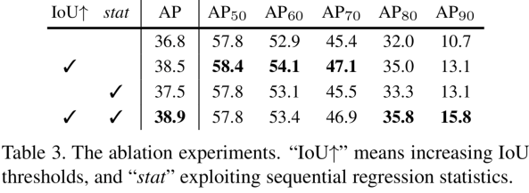


