【Self】Self-Supervised-Learning & BYOL(Bootstrap Your Own Latent)

13 Apr 2021 in Artificial Intelligence

논문 : Bootstrap Your Own Latent
분류 : Self-Training
참고 사이트 :
- Self-training overview: https://hoya012.github.io/blog/Self-Supervised-Learning-Overview/
- BYOL: https://hoya012.github.io/blog/byol/
- BYOL 발표자료: https://www.youtube.com/watch?v=BuyWUSPJicM
- 이전 나의 Post: Self-Supervised-Learning Basics
목차

【DA】ADVENT-Entropy Minimization for DA

11 Apr 2021 in Artificial Intelligence

논문 : ADVENT: Adversarial Entropy Minimization for Domain Adaptation in Semantic Segmentation
분류 : Domain Adaptation
읽는 배경 : Domain Adaptation 기본, Adversarial code의 좋은 예시
느낀점 :
참고 사이트 : Github page,
목차

ADVENT

1. Conclusion, Abstract, Instruction

Task: unsupervised domain adaptation for semantic segmentation
Motivation: Real world와 비교해보면, Data distribution(데이터 분포, 이미지의 통계적 성질)의 많은 차이가 존재한다.
Simple observation
- (1) Source이미지에 대해서, over-confident, low-entropy predictions
- (2) Target이미지에 대해서, under-confident, high-entropy predictions
- 과거에는 Pseudo label을 사용해서 Self-Training을 하는 방법, Feature output에 대해서 Adversarial Learning을 적용하는 방법을 사용했지만, 우리는 Target도 high-confident를 예측하게 만듬으로써, domain gap을 줄이는 방법을 고안했다.
핵심 모듈
- (1) an entropy loss: target 예측 결과가 high-confident 혹은 low-confident 가 되도록 강제한다. 에매하게 [0,1] 중간 값인 0.5 confident를 가지면 Loss를 준다.
- (2) entropy-based adversarial training approach : AdaptSeg가 Output을 이용했다면, 여기서는 Output에 대해서 entropy를 계산한 feature map을 이용해서 Adversarial learning을 적용한다. 이로써, Target 예측결과도 Source 예측 결과처럼 적은 Entropy를 갖도록 유도한다.
- 추가적인 성능향상을 위해서, 아래의 기법을 적용했다.
  - (i) training on specific entropy ranges (Entropy_x_target ∈ [0, 1] (H×W)
  - (ii) incorporating class-ratio priors. (그저 자주 나오는 class가 1 confident가 나와 버리는 문제를 막는다)
성능
- SOTA / Two main synthetic-2-real benchmarks / GTA5 → Cityscapes / SYNTHIA → Cityscapes.

3. Approaches

3.0 Prerequisite

위와 같은 Segmentation Network를 Source data로 학습시킨다,

3.1.1 Direct entropy minimization

위 전체 Architecture에서 상단부분에 있는 모듈이다.
간접적으로는 Domain adaptation이 되도록 만들지만, 엔트로피 관점의 직접적인 최소화 과정이 수행된다.
Target Image에 대해서 high confidence를 추축해내는 F(Network)를 만들어내는 것이 목적이다.
prediction output에 대해서, the Shannon Entropy [36]라는 Entropy를 계산하는 공식을 적용해서 Entropy map을 만들어 낸다.
계산되는 E를 구체적으로 예시를 통해서 알아보자. 아래와 같이 아에 높은 confident, 아에 낮은 confident이여야 낮은 Loss를 얻는다.
위의 그래프에서 x값과 y값의 범위는 각각, [0,1], [0,0.16] 이다. 위 Entropy를 계산해준 후 y값을 [0,1] 사이의 값으로 정규화해준다. 즉 [0, 0.16] -> [0,1]
entropy loss는 soft-assignment version of the pseudo-label이다. 따라서 hard Image dataset에 대해서 좋은 성능을 보여준다. 그리고 threshold를 고르거나 One-hot encoding을 하는 a complex scheduling procedure가 필요없다.
아래의 과정을 통해서 성능을 더욱 끌어올린다.

3.1.2 Self-training = Pseudo Label

3.2 Minimizing entropy with adversarial learning

3.1.1을 보면 c방향으로 sum을 해서 E (W,H)를 구하는 것을 알 수 있다. 이 sum 때문에 자칫하면, 지역에 담긴 구조적인 의존적 의미(? the structural dependencies between local semantics)를 무시할 수 있다. (?)
AdaptSeg가 Output을 이용했다면, 여기서는 Output의 각각의 pixel 스스로의 entropy를 계산한 map(weighted self-information space)을 이용해서 Adversarial learning을 적용한다.
weighted self-information space=I_x : Shape (C x H x W). (단순하게 생각해서, 그냥 각 픽셀마다 이 연산이 수행됐다고 생각하면 되겠다.) 이것을 사용하는 장점은 아래와 같다.
- Source에서 출력되는 I_x 와 Target에서 출력되는 I_x가 유사해지도록 만든다.
- 간접적으로 Entropy를 낮추게 만드는 방법이라고 할 수 있다.
Discriminator, Adversarial Loss, Total Loss이다.

3.3. Incorporating class-ratio priors

위의 방법들 처럼 단순하게 Entropy minimization만 하다보면 한가지 문제점이 생긴다.
그 문제점은 발생 빈도가 높은 class, 쉬운 class를 우선적으로 1로 만들어 버리는 문제이다.
ProDA의 degeneration issue라고 생각하면 된다. 따라서 우리는 regularization 을 하는 과정이 필요하다. (ProDA의 방법이 더 좋을 거다. 아래의 방법은 구식인 것 같다)
아래의 수식을 통해서, Class 발생 빈도 Histogram이 Source와 유사하도록 만든다. 여기서 Mu는 얼마나 유사하게 만들것 인가? 를 나타내는 강도 값이다. 0=약하게, 1=강하게.
the class-prior vector p_s: 각 클래스당 픽셀의 갯수의 L_1 histogram 이다.

4. Experiments

Dataset
- Source: GTA5 or SYNTHIA
- Traget: Cityscape
- DA: 2, 975 unlabeled Cityscapes images are used for trainin
- DA test: Evaluation is done on the 500 validation images
Network architecture
- Deeplab-V
- VGG-16 and ResNet101
- Discriminator in DCGAN [28] : 4conv, leaky-ReLU laye
Implementation detail
- single NVIDIA 1080TI GPU with 11 GB memory
- discriminator: Adam optimizer [19] with learning rate 10−4 to train the discriminator
- 나머지 모델들: SGD with learning rate 2.5 × 10-4 , momentum 0.9 and weight decay 10-4
Weighting factors
- λ_ent = 0.001
- λ_adv = 0.001

5. Results

【Transformer+Video】VisTR & TrackFormer & 3D conv

10 Apr 2021 in Artificial Intelligence

논문1 : End-to-End Video Instance Segmentation with Transformers
논문2 : TrackFormer: Multi-Object Tracking with Transformers
분류 : Video & Tracking + Transformer
느낀점 :
목차

1. VisTR 핵심 및 보충설명

1.1 논문 핵심 정리

Instance segmentation은 하나의 이미지내에서 Pixel-level similarity를 찾내는 Task이다. Instance tracking는 다른 이미지에서 Instance-level similarity를 찾아내는 Task이다. Transformer는 similarity learning에 매우 특화되어 있다. (Why? softmax(Key*Query) 연산을 통해서 구해지는 Attention 값이 결국에는 query와 얼마나 유사한가를 계산하는 것이다)
전체 Architecture는 아래와 같다. 자세한 내용은 PPT에서 찾아보도록 하자.
- 주의할 점으로는, instance queries가 decoder로 들어가서 나오는 최종 결과에 대해서, 각 프레임의 같은 Instance는 같은 i번쨰 query에 의해서 나와야하는 결과들이다. (corresponding indices)
Sequential Network 이기 때문에 발생하는 특징
- Temporal positional encoding (spatial positional encoding 뿐만 아니라, 이것을 3개 뭉친)
- 3D Convolution
36개의 frame이 한꺼번에 들어가므로, 하나의 Sequence of images가 들어가서 총 연산에 걸리는 시간은 조금 걸릴지라도, FPS로 계산하면 상당히 높은 FPS가 나온다.(?)
VisTR가 가지는 특장점들
- instances overlapping를 매우 잘 잡는다 (DETR에서 코끼리 성능 결과 처럼)
- changes of relative positions에도 강하다. (카메라가 고정되지 않아도 된다)
- confusion by the same category instances (비슷한 고릴라, 코끼리 2개 붙어있어도.. 잘 분류하는 편이다)
- instances in various poses 에 대해서 강하다. (사람이 무슨 포즈를 취하든..)
Summary
- a much simpler and faster
- Vedio에 대한 Tracking은 Detection과 Tracking이 따로 진행되기 때문에 이음새가 반듯이 필요한데, VisTR은 seamlessly and naturally 한 모델이다.

1.2. 보충 내용

3D conv란 ??
Dice Loss란? (mask loss를 Focal Loss와 Dice Loss의 합으로 계산된다.)
굳이 Hungarian Loss?? -> 논문을 봐도 내가 생각한게 맞는 것 같다. 최적의 Assignment를 찾기 위해서 Hungarian algorithm을 쓰고, 찾아진 최적의 matching에 대해서만 Loss를 계산하고 backpro 하는 것이다.
Train/Inference Setting
- AdamW, learning rate 10−4, trained for 18 epochs (by 10x at 12 epochs 마다 decays 되는 비율로)
- initialize our backbone networks with the weights of DETR
- 8 V100 GPUs of 32G RAM
- frame sizes are downsampled to 300×540
Faster ??
- 8개 V100 GPU
- ResNet-101 backbone -> 27.7 FPS, Image Process 작업 제외하면 57.7 FPS
- 높은 FPS 원인 (1) data loading을 쉽게 병렬화 처리 할 수 있고 (2) parallel decoding의 가능하고 (3) no post-processing

1.3 코드로 공부해야 할 것들

Temporal Positional Encoding
Mask를 생성하기 위한, the self-attention module.
Self-attetion(O,E)가 B와 Fusion 될때의 연산
Deform_conv

2. VisTR PPT 공부자료

3. TrackFormer 핵심 및 보충설명

3.1 논문 핵심 정리

Key Idea는 track query embeddings을 적용해서, 위의 그림처럼 auto-regressive manner을 사용하는 것이다.
Transformer의 수학적 수식은 위 VisTR 논문 내용과 같다.
전체 순서
1. DETR을 그대로 사용해서, 첫번째 Frame에 대해서 Object Detection을 수행한다.
2. 첫번째 Frame에 대해, Object query에 의해서 나온 Object decoder output 중 object로 판정되는 output을, 다음 Frame의 Object query로 사용한다. (N_track) 뿐만 아니라, 추가적인 N_object query도 당연히 추가한다.
3. 새로운 Frame에 대해서 2번 과정을 반복 수행한다.
4. 학습은 2개의 Frame씩만 묶어서 학습한다.
Track query attention block(= a separate self-attention block) 은 Track queries 끼리 서로 소통하게 만드는 모듈이다. (위 이미지 아래 모듈) 이 모듈을 통해서 t-1 Frame의 Object 위치와 구조에 대한 정보를 그대로 사용하는게 아니게 만들어서, 새로운 Frame에 대한 적응을 좀더 잘하게 만들어 주었다.
신박한 학습 기법들
1. t-1 Frame을 t 주변의 아무 다른 Frame으로 대체해서 학습시킨다. 객체의 포즈나 위치가 확확 바뀌는 상황에도 잘 적응하게 만들기 위함이다.
2. 어떠한 query type(track, object)에서도 잘 반응할 수 있게 만들기 위해서, 가끔 track query를 제거해서 다음 Frame Decoder에 넣어준다. 학습 밸런싱을 맞추는 과정이다. 새로 나타난 객체에 대해서도 잘 Detecion 하게 만들어 주는 방법이다.
3. Track queries에 Background에 대한 output도 넣어준다. (내 생각으로 이 과정을 통해서, Track query attention block 과정을 통해서 object occlusion의 문제점을 완화시켜준다.)
DETR에서 Panoptic Sementation 구조를 그대로 차용해서 Instance에 대한 Mask 예측도 수행하고, MOTS 결과도 출력해보았다.

3.2. 보충 내용

Bipartite track query matching에 대한 부분
MOT dataset, Environment Setting에 대해서는 추후에 필요하면 공부해보자.

4. TrackFormer PPT 공부자료

【DA】AdaptSegNet-Learning to Adapt Structured Output Space

10 Apr 2021 in Artificial Intelligence

논문 : Learning to Adapt Structured Output Space for Semantic Segmentation
분류 : Domain Adaptation
읽는 배경 : Domain Adaptation 기본, Adversarial code의 좋은 예시
느낀점 :
참고 사이트 : Github page

AdaptSegNet

Deeplab V2를 사용했다고 한다. V2의 architecture 그림은 없으니 아래의 V3 architecture 그림 참조
AdaptSegNet 전체 Architecture
코드를 통해 배운, 가장 정확한 학습과정 그림은 해당 나의 포스트 참조.

1. Conclusion, Abstract

DA semantic segmentation Task를 풀기 위해, adversarial learning method을 사용한다.
방법1 : Adversarial learning을 사용한다. in the output space(last feature map, not interval feature map)
방법2 : 위의 그림과 같이 a multi-level에 대해서 adversarial network 을 사용한다. multi-level을 어떻게 사용하는지에 대해서는 위의 Deeplab V3 architecture를 참조할 것.
방법1의 Motivation : 아래 그림과 같이, 이미지 사이에는 많은 차이가 있지만, CNN을 모두 통과하고 나온 Output feature map은 비슷할 것이다.
- 따러서 Sementic segmentation의 예측결과 output을 사용하여, Adversarial DA과정을 진행함으로써, 좀더 효과적으로 scene layout과 local contect를 align할 수 있다.

2. Instruction, Relative work

pass

3. Method

the discriminator D_i (level i): source 이미지로 부터온 prediction Ps인지 Target, 이미지로 부터온 prediction Pt인지 구별한다.
target prediction에 대한 Adversarial loss를 적용해서, G(Generator=Feature encoder)가 similar segmentation distribution를 생성하게 만든다.
Output Space Adaptation에 대한 Motivation
1. 과거의 Adversarial 방법들은, 그냥 feature space(맨 위 이미지에서 빨간색 부분=complex representations)를 사용해서 Adversarial learning을 적용했다.
2. 반면에, segmentation outputs(맨위 이미지에서, hard labeling 작업 이전의 최종 예측 결과값)은low-dimension이지만 rich information을 담고 있다.
3. 우리의 직관으로 이미지가 source이든 target이든 상관없이, segmentation outputs은 굉장히 강한 유사성을 가지고 있을 것이다.
4. 따라서 우리는 이러한 직관과 성질을 이용해서, low-dimensional softmax outputs을 사용한 Adversarial Learning을 사용한다.
Single-level Adversarial Learning: 아래 수식들에 대해서 간단히 적어보자
1. Total Loss
2. Discriminator Loss: Discriminator 만들기
3. Sementic segmentation prediction network
4. Adversarial Loss: Generator(prediction network)가 target 이미지에 대해서도 비슷한 출력이 나오게 만든다
Multi-level Adversarial Learning
- Discriminator는 feature level마다 서로 다른 Discriminator를 사용한다
- i level feature map에 대해서 ASPP module(pixel-level classification model)을 통과시키고 나온 output을 위 이미지의 (2),(3),(4)를 적용한다.
Network Architecture and Training
1. Discriminator
  - all fully-convolutional layers, convolution layers with kernel 4 × 4 and stride of 2, channel number is {64, 128, 256, 512, 1},
  - leaky ReLU parameterized by 0.2
  - do not use any batch-normalization layers: small batch size를 놓고 각 source batch, target batch 번갈아가면서 사용했기 때문이다.
2. Segmentation Network
  - e DeepLab-v2 [2] framework with ResNet-101 [11] model
  - modify the stride of the last two convolution layers from 2 to 1 함으로써, 최종결과가 이미지 H,W 각각이 H/8, W/8이 되도록 만들었다.
  - an up-sampling layer along with the softmax output
3. Multi-level Adaptation Model
  - we extract feature maps from the conv4 layer and add an ASPP module as the auxiliary classifier
  - In this paper, we use two levels.
  - 위 그림을 보면 이해가 쉽니다.
4. Network Training(학습 과정)
  1. (Segmentation Network와 Discriminators를 효율적으로 동시에 학습시킨다.)
  2. 위의 Segmentation Network에 Source 이미지를 넣어서 the output Ps를 생성한다.
  3. L_seg를 계산해서 Segmentation Network를 Optimize한다.
  4. Segmentation Network에 Target 이미지를 넣어서 the output Pt를 생성한다.
  5. Optimizing L_d in (2). 위에서 만든 Ps, Pt를 discriminator에 넣고 학습시킨다.
  6. Adversarial Learning : Pt 만을 이용해서 the adversarial loss를 계산하여, Segmentation Network를 Adaptation 시킨다.
5. Hardware
  - a single Titan X GPU with 12 GB memory
  - the segmentation network
    - Stochastic Gradient Descent (SGD) optimizer
    - momentum is 0.9 and the weight decay is 5×10−4
    - initial learning rate is set as 2.5×10−4
  - the discriminator
  - Adam optimizer
  - learning rate as 10−4 and the same polynomial decay
  - The momentum is set as 0.9 and 0.99

4. Results

성능 결과 및 Ablation study에 대한 내용은 Pass

【Pytorch】 mmclassification teardown reports & Ubuntu re-install

09 Apr 2021 in Pytorch / Docker / Git

Ubuntu re-install & mmclassification teardown reports

1. New ubuntu setting List

우분투 설치
gpu graphic driver 설치
docker, docker-nvidia 설치
Vscode 설치
anaconda 설치
docker image, container 필요한거 다운 및 설치 (MLworkspace, pytorch-cuda)
dataset 다운로드 (coco, imagenet)

2. Docker setting

Docker hub naming (참고 사이트)
- devel : 속편하지만 용량이 너무 큼
- base : 가장 낮은 용량
- runtime : 사용하기에 적절한 용량
- 이유는 모르겠지만 pytorch-1.5.1-cuda10.1-runtime에서는 cat /usr/local/cuda/version.txt가 동작하지 않는다. 그럼에도 불구하고 예전에 detr을 cuda로 돌렸었다. mmclf에서는 cuda문제가 발생했으므로 속편하게 pytorch-1.5.1-cuda10.1-devel 사용해야겠다.
docker run –shm-size
- shared memory 사용 공간 ML-workspace에서 512MB를 주니, 대충 그정도 사용하면 될 듯하다.

docker run

detr에서 준 dockerfile을 build해서 사용했다. 하지만 cuda 문제가 발생했다.
detr에서 준 docker image 부터가 잘못 됐다. 재설치 필요
docker hub - pytorch 1.5.0 - devel 을 사용한다. runtime에는 cat /usr/local/cuda/version.txt 가 동작하지 않는다. 맘편하게 devel사용한다.
아래와 같이 -v를 2번 가능하다. <my path>/<container path> 에서, <container path>는 path가 존재하지 않으면 자동으로 mkdir된다.

$ sudo docker run -d -it      \
--gpus all         \
--restart always     \
-p 8000:8080         \
--name "mmcf"          \
--shm-size 2G      \
-v ./home/junha/docker/mmclf/mmclassification   \ # 가능하면 무조건 절대경로 사용할 것
-v /hdd1T:/dataset   \
pytorch/pytorch:1.5.1-cuda10.1-cudnn7-devel
  
$ sudo docker run -d -it      \
--gpus all         \
--restart always     \
-p 8080:8080         \
--name "mmcl"          \
--shm-size 2G      \
-v /home/junha/docker:/workspace  \
-v /hdd1T:/dataset   \
sb020518/mmcl:0.1

3. mm installation

mmcv installation

$ apt-get update
$ apt-get install ffmpeg libsm6 libxext6  -y
$ pip install mmcv-full==1.3.0 -f https://download.openmmlab.com/mmcv/dist/cu101/torch1.5.0/index.html

mmclasification install

$ git clone https://github.com/open-mmlab/mmclassification.git
$ cd mmclassification
$ pip install -e .  # or "python setup.py develop"

이런 식으로 install하면, 이 공간의 mmcls 파일을 수정하면, import mmcls.util.collect_env 이것을 새로운 py파일에 적든, 터미널에서 python을 실행해서 적든, 모두 수정된 코드 내용이 적용 된다.

mmclasification install Test

python demo/image_demo.py \
/workspace/checkpoints/dog.jpg  \
/workspace/configs/resnet/resnet50_b32x8_imagenet.py  \
/workspace/checkpoints/resnet50_batch256_imagenet_20200708-cfb998bf.pth 

4. 코드 공부 흐름 필수

~~Github 패키지 이곳저곳 돌아다니면서, 전체적인 구조 눈으로 익히기(좌절하기 말기. 핵심만 파악하려 노력하기)~~
~~Interence 흐름 따라가기~~
~~Tranin 흐름 따라가기~~
~~Dataloader 공부하기~~
~~Loss, Optimizer, Scheduler 분석하기~~
~~Model save load, check point 분석하기~~
~~Batch 구성방법, GPU 분산학습 분석하기~~

[코드에서 다 봐야하는 것] (순서대로 보지 말고. 코드 따라가면서 눈에 보이는 것 부터 부셔버리기)

Github로 전체적인 구조 눈으로 익히기
Interence 흐름 따라가기
Tranin 흐름 따라가기
Dataloader 공부하기
Loss, Optimizer, Scheduler 분석하기
Model save load, check point 분석하기
Batch 구성방법, GPU 분산학습 분석하기

5. mmclassification github

Python argparse 사용법
- parser.add_argument에 대해서, –가 붙여 있는 것은 optional 이다. –가 없는 것은 필수입력인자(positional) 이다.
- add_argument()에 들어가는 인자가 많다.
- 그 인자 중, type= 설정해주지 않으면 str이 default
- 그 인자 중, default= 값이 지정되지 않았을 때, 사용할 디폴트값
config 파일 분석하기 (아래 팁 참조)
- configs/resnet/resnet50_b32x8_imagenet.py에는 또 다른 config 파일의 path만 기록 되어 있다.
- 어려울 거 없이, 그 path의 config 파일만 다~ 모아서 cfg에 저장된다.
- 이쁘게 출력해보고 싶으면, print(f'Config:\n{cfg.pretty_text}')
test.py이든 train.py이든 핵심 호출법은 아래와 같다.
- model: model = build_classifier(cfg.model)
- dataset: dataset = build_dataset(cfg.data.test), datasets = [build_dataset(cfg.data.train)]

6. mmclassification/getting_started.md

Prepare datasets
- ImageNet 다운로드. 각 클래스는 같은 폴더에 넣어주기 위한 sh 실행 (참조사이트).
- MNIST, CIFAR10 and CIFAR100와 같은 데이터 셋은, 만약 데이터셋이 없다면 자동으로 다운 받아진다.
Inference a dataset
- Inference는 이미지를 모델이 넣고 나오는 결과를 직접 눈으로 확인해보는게 목적이다.
- mmclassification에서는 inference.py 파일 없다.
- 굳이 하고 싶다면, demo/image_demo.py를 이용하자.
Test a datatset
- Test는 val_img들에 대해서 예측결과를 추론해보는 것이 목표이다.
- tools/test.py, tools/dist_test.sh
- dist_test.sh는 결국 tools/test.py 실행한다.
- $ python tools/test.py ${CONFIG_FILE} ${CHECKPOINT_FILE} [--out ${RESULT_FILE}] 이거로 먼저 debuging하고 그 다음에 dist_test.sh 파일을 이용해서 multi-gpu testing을 진행하자.
- $ python tools/test.py configs/resnet/resnet50_b32x8_imagenet.py checkpoints/resnet50_batch256_imagenet_20200708-cfb998bf.pth --out result/imagenet-val.json
Train a dataset
- $ python tools/train.py configs/resnet/resnet50_b32x8_imagenet.py --load-from checkpoints/resnet50_batch256_imagenet_20200708-cfb998bf.pth

7. tools/test.py 디버깅

이제부터 아래의 과정은 디버깅을 통해 알아낸 내용이다,
[Vscode Debugging] : tools/test.py + "args" : ["configs/resnet/resnet50_b32x8_imagenet.py", "checkpoints/resnet50_batch256_imagenet_20200708-cfb998bf.pth "], or "args" : ["configs/resnet/resnet50_b32x8_imagenet.py", "checkpoints/resnet50_batch256_imagenet_20200708-cfb998bf.pth", "--metrics", "mAP", "CP", "CR"]
[Terminal] : python tools/test.py configs/resnet/resnet50_b32x8_imagenet.py checkpoints/resnet50_batch256_imagenet_20200708-cfb998bf.pth --out ./result/imagenet-val-resnet50.json --metrics "accuracy" "precision" "recall" "f1_score" "support"

build_dataset/classifier 호출 순서

# 아래로 내려갈 수록 define으로 들어가는 것
   
## 1. dataset
from mmcls.datasets import build_dataloader, build_dataset
from mmcv.utils import Registry, build_from_cfg
return <class 'mmcls.datasets.imagesnet.ImagesNet'> # cfg.dataset_type 에 적힌 class
# return이 완벽하게 되기 이전에 __init__ 가 실행되면서, 맴버 변수가 채워진다. 이때 pipeline(augmentation)이 정의된다.
   
## 2. classifier
from mmcls.models import build_classifier
from mmcv.utils import build_from_cfg
return <class 'mmcls.models.classifiers.image.ImageClassifier'> # cfg.model.type 에 적힌 class
# return이 완벽하게 되기 이전에 __init__ 가 실행되면서, 맴버 변수가 채워진다. 이떄 backbone, neck, head가 정의된다. 

mmcls.datasets.imagesnet.ImagesNet
mmcls.models.classifiers.image.ImageClassifier
최종 test.py의 108 line까지 실행된 결과

model.eval() 하고, 테드스 결과 뽑아내기
```
# tools/test.py
model = MMDataParallel(model, device_ids=[0])
outputs = single_gpu_test(model, data_loader)
```
- mmcv/paralled/MMDataParalle == from torch.nn.parallel import DataParallel
- 여기서 model = <class 'mmcv.paralled.MMDataParalled' object> 로 바뀐다.
- dataloader = <class 'torch.utils.data.dataloader.DataLoader' object>

result 결과 뽑기

# from mmcls.apis import single_gpu_test
for i, data in enumerate(data_loader):
        with torch.no_grad():
            result = model(return_loss=False, **data)
               
"""
type(result) = list 
len(result) = 32 = batch size = cfg.data.samples_per_gpu
type(result[0]) = numpy.ndarray
result[0].shape = (1000,)
"""

8.tools/train.py 디버깅

argparse, config 읽고, 에러 미리 확인.

build_ 수행하기

model = build_classifier(cfg.model)
datasets = [build_dataset(cfg.data.train)]
# cpu worker 처리만 해주고
train_model(
        model,
        datasets,
        cfg,
        distributed=distributed,
        validate=(not args.no_validate),
        timestamp=timestamp,
        meta=meta)

from mmcls.apis import train_model

# /mmcls/apis/train_model
"""
1. dataloader = `<class 'torch.utils.data.dataloader.DataLoader' object>
2. model = `<class 'mmcv.paralled.MMDataParalled' object>
"""
runner = build_runner(
        cfg.runner,
        default_args=dict(
            model=model,
            batch_processor=None,
            optimizer=optimizer,
            work_dir=cfg.work_dir,
            logger=logger,
            meta=meta))
   
runner.run(data_loaders, cfg.workflow)

build_runner= <mmcv.runner.epoch_based_runner.EpochBasedRunner> (Github link)
runner.run (Github link)

from mmcv.runner import epoch_based_runner

아래 코드는, 아래로 차근차근 내려가면서 실행된다고 보면 된다.

# /mmcls/runner/epoch_based_runner
class EpochBasedRunner(BaseRunner):
    def run(self, data_loaders, workflow, max_epochs=None, **kwargs): # kwargs = {None}, self.model 이미 저장되어있음
        epoch_runner = getattr(self, mode) 
    	epoch_runner(data_loaders[i], **kwargs) 
        # == self.train(data_loaders[i], **kwargs)
    def train()
        for i, data_batch in enumerate(self.data_loader):
            self.run_iter(data_batch, train_mode=True)
    def run_iter(self, data_batch, train_mode, **kwargs):
         outputs = self.model.train_step(data_batch, self.optimizer, **kwargs)
               
"""
여기서 model은 
<class 'mmcls.models.classifiers.image.ImageClassifier' object> 이자
<class 'mmcv.paralled.MMDataParalled' object> 이다. 
따라서 아래의 파일에 들어가면 ""train_step"" 함수 찾기 가능!
"""   

mmclassification/mmcls/models/classifiers/base.py

# mmclassification/mmcls/models/classifiers/base.py
class BaseClassifier(nn.Module, metaclass=ABCMeta):
    def train_step(self, data, optimizer):
        losses = self(**data) #== BaseClassifier.fowerd 실행!
        outputs = dict(loss=loss, log_vars=log_vars, num_samples=len(data['img'].data))
    def forward(self, img, return_loss=True, **kwargs):
        if return_loss:
            return self.forward_train(img, **kwargs)
       
def forward_train(self, imgs, **kwargs):
	pass
    # 즉! torch.nn.Module.forward 그대로 실행된다.

중요하지만, 사소한 추가 팁들 모음

1. config 파일 넌 무엇인가?!

# test.py에서 디버깅 하면서, cfg파일 읽어보기 
print(f'Config:\n{cfg.pretty_text}')

########## 예를 들어서 이 파일을 봐보자. configs/resnet/resnet50_b32x8_imagenet.py  ##########
_base_ = [
    '../_base_/models/resnet50.py', '../_base_/datasets/imagenet_bs32.py',
    '../_base_/schedules/imagenet_bs256.py', '../_base_/default_runtime.py'
]

########## '../_base_/models/resnet50.py'  ##########
model = dict(
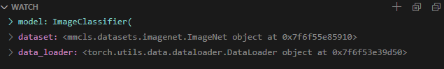
    type='ImageClassifier',
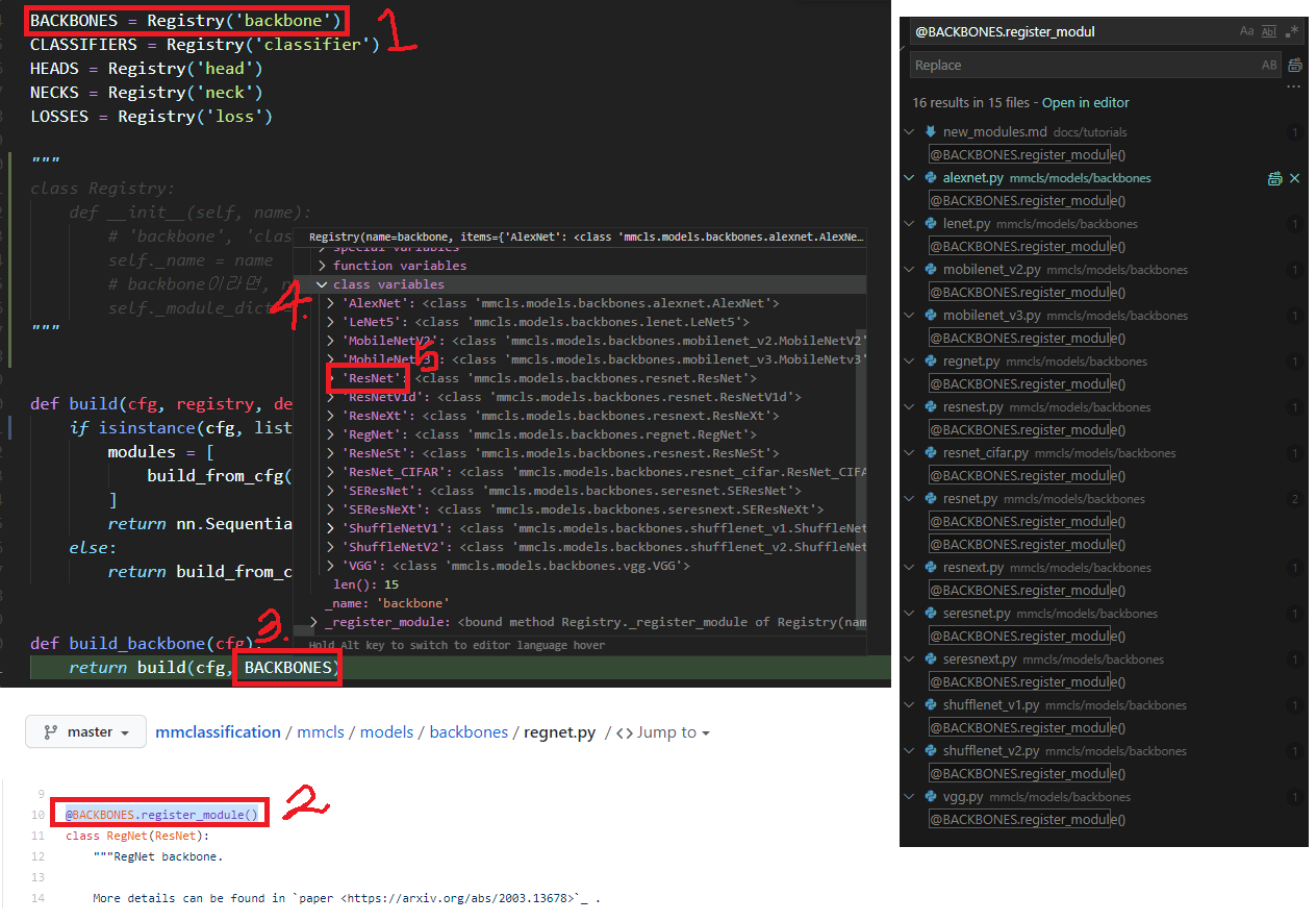
    backbone=dict(
        type='ResNeSt',
        depth=50,
        num_stages=4,
        out_indices=(3, ),
        style='pytorch'),
    neck=dict(type='GlobalAveragePooling'),
    head=dict(
        type='LinearClsHead',
        num_classes=1000,
        in_channels=2048,
        loss=dict(type='CrossEntropyLoss', loss_weight=1.0),
        topk=(1, 5),
    ))


########## '../_base_/datasets/imagenet_bs32.py'  ##########
dataset_type = 'ImageNet'
img_norm_cfg = dict(
    mean=[123.675, 116.28, 103.53], std=[58.395, 57.12, 57.375], to_rgb=True)
# 원하는 Transformer(data agumentation)은 아래와 같이 추가하면 된다.
train_pipeline = [
    dict(type='LoadImageFromFile'),
    dict(type='RandomResizedCrop', size=224),
    dict(type='RandomFlip', flip_prob=0.5, direction='horizontal'),
    dict(type='Normalize', **img_norm_cfg),
    dict(type='ImageToTensor', keys=['img']),
    dict(type='ToTensor', keys=['gt_label']),
    dict(type='Collect', keys=['img', 'gt_label'])
]
test_pipeline = [
    dict(type='LoadImageFromFile'),
    dict(type='Resize', size=(256, -1)),
    dict(type='CenterCrop', crop_size=224),
    dict(type='Normalize', **img_norm_cfg),
    dict(type='ImageToTensor', keys=['img']),
    dict(type='Collect', keys=['img'])
]
# 위에 내용은 이 아래를 정의하기 위해서 사용된다. cfg.data.test, cfg.data.val 이 사용된다.
data = dict(
    samples_per_gpu=32,
    workers_per_gpu=2,
    train=dict(
        type=dataset_type,
        data_prefix='data/imagenet/train',
        pipeline=train_pipeline),
    val=dict(
        type=dataset_type,
        data_prefix='data/imagenet/val',
        ann_file='data/imagenet/meta/val.txt',
        pipeline=test_pipeline),
    test=dict(
        # replace `data/val` with `data/test` for standard test
        type=dataset_type,
        data_prefix='data/imagenet/val',
        ann_file='data/imagenet/meta/val.txt',
        pipeline=test_pipeline))
 evaluation = dict(interval=1, metric='accuracy')


########## '../_base_/schedules/imagenet_bs256.py'  ##########
optimizer = dict(type='SGD', lr=0.1, momentum=0.9, weight_decay=0.0001)
optimizer_config = dict(grad_clip=None)
# learning policy
lr_config = dict(policy='step', step=[30, 60, 90])
runner = dict(type='EpochBasedRunner', max_epochs=100)


########## '../_base_/default_runtime.py'  ##########
# checkpoint saving
# 1번 epoch씩 모델 파라미터 저장
checkpoint_config = dict(interval=1)
# yapf:disable
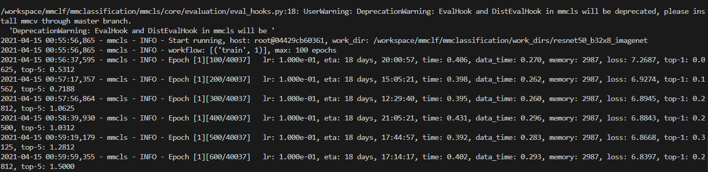
# 100번 iteration에 한번씩 log 출력 
log_config = dict(
    interval=100,
    hooks=[
        dict(type='TextLoggerHook'),
        # dict(type='TensorboardLoggerHook')
    ])
# yapf:enable
dist_params = dict(backend='nccl')
log_level = 'INFO'
load_from = None
resume_from = None
workflow = [('train', 1)] # [('train', 2), ('val', 1)] means running 2 epochs for training and 1 epoch for validation, iteratively.

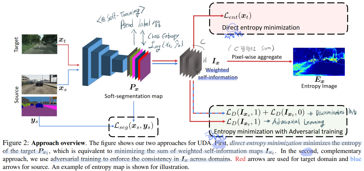
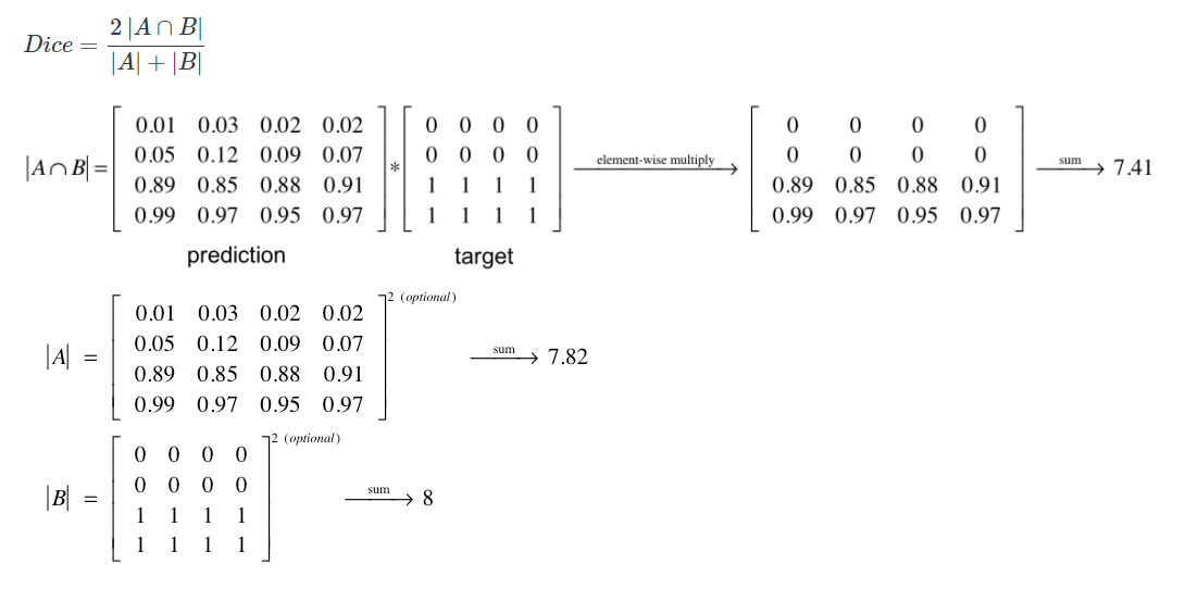
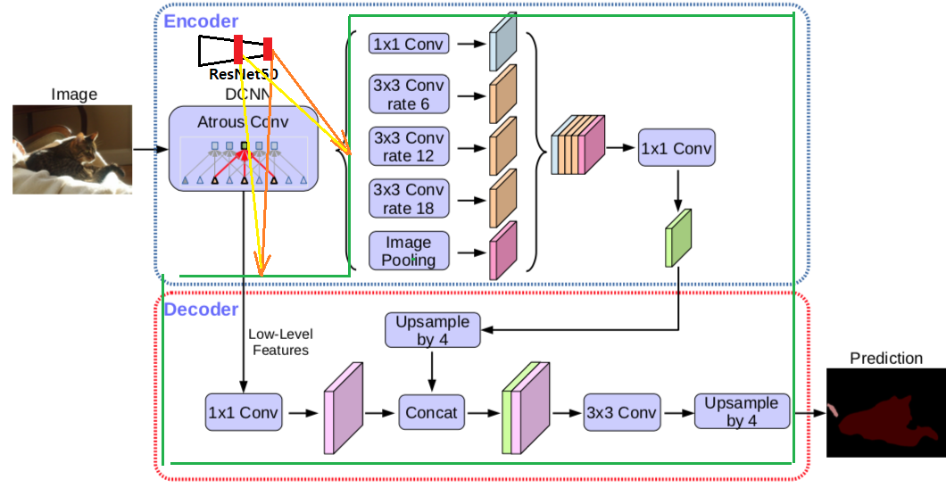
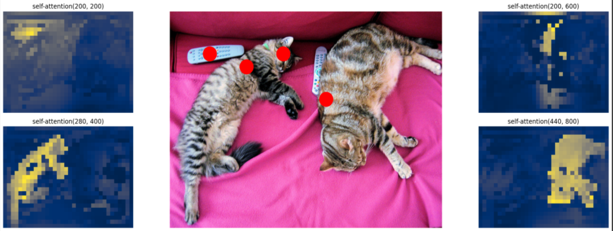
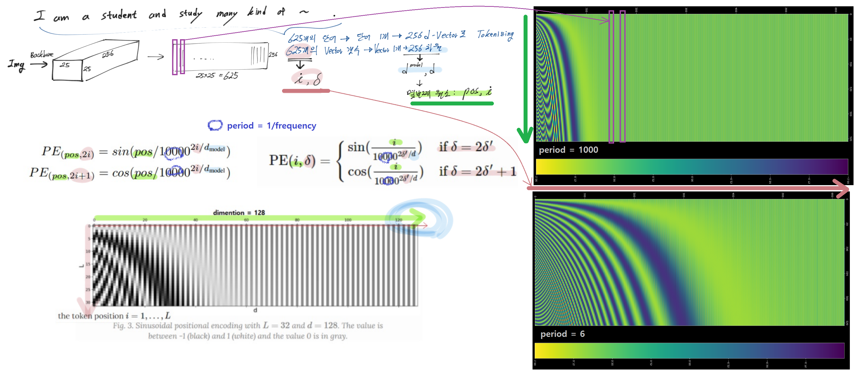
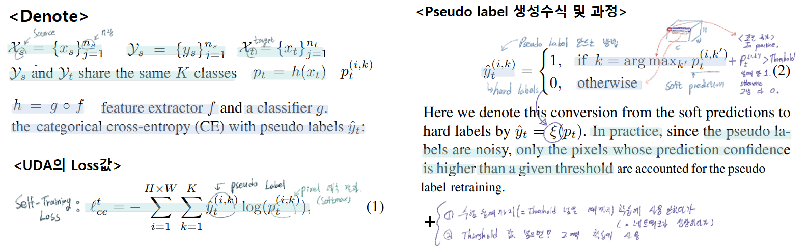
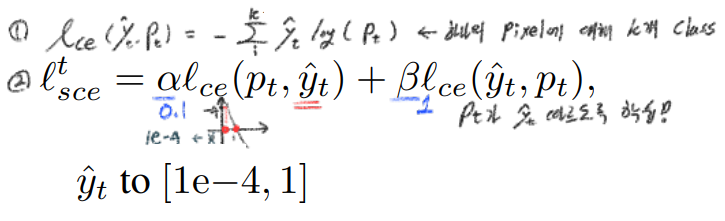
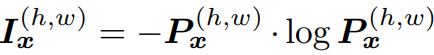
2. Registry는 모두 안다. 난 고르기만 하면 된다.

mmcv.utils.Registry 사실 맴버 변수는 2개 뿐이다,
self._name = ‘backbone’
self._module_dict = 아래 그림 4번처럼 모든 backbone을 다 알고 있다!! 어떻게 알지??
아래 그림 2번과 같이 정의된 class를 모두 담고 있는 것이다.
@BACKCONES.register_modules()* 은 언제 실행되는 것 일까? 초반에 import할때 모두 실행된다. 여기*에다가 Breakpoint 걸고 디버깅한 결과는 아래와 같다.
```
# test.py
import mmcls.models
import mmcls.models.__init__
import mmcls.models.backbone.__init__
from .regnet import RegNet
```

3. checkpoint = load_checkpoint(model, args.checkpoint) 결과는?

type( checkpoint ) = dictionary
Netron 이용해서 Visualization 하자

4. 모델 파라미터 가져오기 - “어차피 텐서다 쫄지말자”

How to load part of pre trained model?

pretrained_dict = ...
model_dict = model.state_dict()
  
# 1. filter out unnecessary keys
pretrained_dict = {k: v for k, v in pretrained_dict.items() if k in model_dict}
# 2. overwrite entries in the existing state dict
model_dict.update(pretrained_dict) 
# 3. load the new state dict
model.load_state_dict(pretrained_dict)

5. mmcls/models/backbones/ResNet.py forward 를 실행하기 까지의 과정은?

tools/test.py의 가장 마지막이, single_gpu_test 함수에 들어가는 것이었다.
mmcls/models/backbones/ResNet.py 에다가 breakpoint 걸어서 디버깅 해본 결과, 아래와 같은 코드 흐름을 확인할 수 있었다.
알아만 두자.

6. python getattr()

# mmcv.runner.epoch_based_runner.py
# ** 아래의 2 코드는 같은 말이다. ** if mode == str('train') **
epoch_runner = getattr(self, mode) 
epoch_runner = self.train()

따라서 디버깅으로 EpochBasedRunner을 확인해보면 train 맴버함수 (Github link)를 가지고 있는 것을 알 수 있다.

【Pytorch】 DETR code teardown reports / 핵심 배운점 2개

06 Apr 2021 in Pytorch / Docker / Git

DETR github : https://github.com/facebookresearch/detr
Remarks
1. Dockerfile 제공 (사용하지 말기)
2. Demo code 제공
한글 주석 포함 github 링크
- https://github.com/junha1125/DETR-with-Kcomment
- data 폴더 제외 cp 명령하기 $ cd ~/DETR-with-Kcomment && rsync -av --progress /workspace/* ./ --exclude 'coco'

의문 정리 (검색하기)

demo에서 0.1을 왜 곱해주지??
coco_evaluator 를 어떻게 사용하는건지 패스했다. 나중에 공부해보자.

multihead attention에서 width height가 계속 다르게 들어가는데, W(linear)를 어떻게 학습시키지? linear도 input, output dimension을 고정시켜줘야 할 텐데…

굳이 이해하려 하지말고, torch.nn.MULTIHEADATTENTION 그대로 사용하자.
vector의 갯수는 상관없다. 그냥 key, value 적당한 차원으로 넣어주면 된다.

예를 들어서 아래와 같은 코드가 있다. 아래에 주석 참조!

class TransformerEncoderLayer(nn.Module):
    def __init__(self, d_model=512, nhead=8, dim_feedforward=2048, dropout=0.1,
                 activation="relu", normalize_before=False):
        super().__init__()
        self.self_attn = nn.MultiheadAttention(d_model, nhead, dropout=dropout)
        self.linear1 = nn.Linear(d_model, dim_feedforward) 
        # (512 -> 2048) x (feature_map width x height) 이 모든 것에 같은 linear 연산이 이뤄진다.
        # self.linear1의 weight.shape = 512x2048 
              
    def forward_post(self,
        q = k = self.with_pos_embed(src, pos)
        src2, score = self.self_attn(q, k, value=src, attn_mask=src_mask,
                              key_padding_mask=src_key_padding_mask)
        src = src + self.dropout1(src2)
        src = self.norm1(src)
        # 2. Feed Forward
        src2 = self.linear2(self.dropout(self.activation(self.linear1(src))))

의문 해결
- detr.py에 num_classes = 91 if args.dataset_file != 'coco' else 20 를 num_classes = 20 if args.dataset_file != 'coco' else 91 로 바꾸면, 왜 main.py 에서 디버깅 실행하면 from models import build_model 에서 에러가 나는 거지? 에러내용은 아래 사진 (해결 - 반성하자)
추신
- 아래의 목차 순서 잘 분리해놓았으니, 무시하지 말고 꼭 신경쓰기

0. 핵심 배운점

0.1 디버깅 배운점 (1)

나의 현재 문제점
1. 코드(main.py)를 처음부터 똑바로 안봤다. torch.utils.data.dataset이 아니라, build_dataset이었는데.. 아무 생각 없이 패스했다.
2. dataloader의 파라미터 중에서 collate_fu이 정말 중요했는데, 이것도 무시했다.
3. 이건* 나중에 보자!라는 마음으로 패스하고, 나중에 그걸* 안봐서 너무 힘들었다.
4. 내가 지금 뭐하지는 모르고 계속 했던거 또하고 했던거 또했다.
해결책
1. 정말 하나하나! 꼼꼼히! 순서대로! 부셔야 한다.
2. 그냥 아무 생각없이 디버깅 하기 전에 아래의 방법** 중 지금의 에러를 해결하기 위해 사용해야하는 방법이 무엇인지 진지하게 생각하고! 들어가자. 손부터 움직이지 말고 머리를 쓰자.
3. 좌절하지 말자. 포기하지 말자. 할 수 있다. 아자아자
최적의 디버깅 방법**이 무엇인가?
- 코드 직접 수정하기
- pdb 이용하기 / pdb의 interact 이용하기
- python debuger 이용하기 / Watch, Debug console이용하기
- 코드 전체에서 (특정 클래스, 함수) 검색해보기 / VScode의 define(F12)과 reference(shift+F12) 잘 이용하기
- (위의 방법 섞기)
- 코드를 직접 수정하기 + pdb이용하기
- 코드를 직접 수정하기 + Python debuger를 이용하기
신경망에 있어서 디버깅 방법
- __init__ 과 forward가 실행되는 시간 차는 매우 다르다. 따라서 분리해서 생각하도록 하자.
- forward는 for x,y in data_loader: 이후에 실행이 된다. 그 이전에 model을 build하는 과정에서는 모두 __init__만 실행된다.
추가 꿀팁
1. 뭔가 안된다면, worker = 1 로 해놓고 디버깅 할 것.
2. 왜 안되는지 앞으로 따라가 보고, 앞으로 따라가도 모르겠으면
3. 뒤로 가야한다. 뒤로가서 무엇을 하고 나서 이상이 생긴건지.

0.2 개발자로써 배운점 (2)

4일 동안 DETR 코드를 하나하나 씹어먹으며 공부하다가, 결국 나는 아래와 같은 큰~~!! 깨달음을 얻었다.
코딩 공부는 고등학교 시험공부, 대학교 시험공부 처럼 하는게 아니다.
Just Do It. 뭐든 만들어 보고, 뭐든 시도해봐야한다. (by nomadcoders 니꼬쌤 . 나의 동기, 선배님!)
따라서! 아래와 같은 생각은 틀렸다. 그냥 100프로 틀렸다.
- 모든 것 하나하나 다 부셔버리고, 다 알고 넘어가야 한다.
- 기초부터 차근차근 모두 다 알아야 한다.
- 나중에 내가 스스로 만들 수 있게 충분히 이해해야 한다.
- 언젠간 내가 처음부터 끝까지 만들 수 있어야 한다.
이게 아니고! 아래와 같이 생각하는게 정답이다. 이게 무조건 맞다. 100프로 이다.
- 그냥 사용할 수 있으면 장땡이다. 대충 그런것 같은데… 라고 input 넣어서 원하는 output 얻었으면 끝! 더 이상 볼 필요도 없다.
- 왜냐면 어차피 그 함수, 프레임워크 미친듯이 공부하고 완벽히 이해했다고 해도, 곧! 언젠가! 그 함수 프레임워크 보다 좋은게 나온다.
- 그럼 내가 기초부터 쌓았다고 좋아했던 모든 시간들이 쓰레기가 된다.
- 개발자는 기초 따위는 중요하지 않다. 파이썬 쓰면서 C언어 안 보잖아. numpy쓰면서 그 안에 어떻게 돌아가는지 몰라도 되잖아. 기초가 중요하다는 소리는 이제 나에게 필요없는 소리다.
- 빨리 무언가 만들어보고 실험해보는 자세가 앞으로 개발자로써 내가 가져야 하는 진짜 자세이다.
- 패키지는 내가 만드는게 아니다. 내가 해야할 것은 남이 만든 패키지를 이리저리 섞는 것이다. 남이 만든 패키지도 결국 누군가가 만들어 놓은 것을 융합해놓은 것일 뿐이다.
- ‘이러한 기능을 하는 함수/클래스가 필요한데..’ 라는 생각이 들면, 패키지를 처음부터 끝까지 공부하면서 그 함수/클래스를 찾아야 하는게 아니라, 많은 패키지에서 그 함수와 클래스를 (랜덤적으로 뒤져보면서) 결국 찾아내서 사용하기만 하면 끝이다.
- 정신 차려라 개발자가 기초를 생각하기엔 쇠퇴 및 발전 속도는 미치도록 빠르다.

1. detr_demo.py. Inference 흐름 따라가기

Github/facebookresearch/detr Code link

Error 해결

$ pip install torch==1.5.0+cu101 torchvision==0.6.0+cu101 -f https://download.pytorch.org/whl/torch_stable.html 
# docker Image 그대로 사용했어야 했다. requirements.txt가 개세끼다
$ conda install -c conda-forge ipywidgets
$ pip install pdbpp

주요 코드 설명
1. h = self.transformer(pos + 0.1 * h.flatten(2).permute(2, 0, 1), self.query_pos.unsqueeze(1)).transpose(0, 1)
  - 위의 transformer 함수 내부 : ((625, 1, 256) + 0.1 * (625(갯수), 1, 256(백터) , (100, 1 ,256)) : 0.1을 왜 곱해주지??
  - transformer ouput : (100, 1 ,256)
  - h.shape : (by transpose) : (1, 100, 256)
이 코드는 nn.transformer를 그대로 사용하기 때문에.. 여기서 그만 공부..

SmartSelect_20210418-161421_Samsung Notes.jpg

2. Evaluation. Inference 흐름 따라가기

main.py는 train.py 코드도 되고, test.py 코드도 된다. --eval 옵션만 넣고 빼주면 된다.

[Terminal]
$ python main.py \
		--batch_size 1\
        --no_aux_loss\
        --eval\
        --resume https://dl.fbaipublicfiles.com/detr/detr-r50-e632da11.pth
        --coco_path /workspace/coco # /path/to/coco

$ python main.py \
       	--batch_size 2\
        --no_aux_loss\
        --eval\
        --resume checkpoints/detr-r50-e632da11.pth\
        --num_workers 4\
        --world_size 2\
        --coco_path /dataset/coco\
        --output_dir result

[Vscode Debugging] 
# ./vscode/launch.json
"args" : ["--batch_size", "2", 
        "--no_aux_loss", 
        "--eval", 
        "--resume", "checkpoints/detr-r50-e632da11.pth", 
        "--num_workers", "4",
        "--world_size", "2",
        "--coco_path", "/dataset/coco",
        "--output_dir", "result"]

2.0 `main.py` 분석해보기

print(args)

- Namespace(aux_loss=False, backbone='resnet50', batch_size=1, bbox_loss_coef=5, clip_max_norm=0.1, coco_panoptic_path=None, coco_path='/workspace/coco', dataset_file='coco', dec_layers=6, device='cuda', dice_loss_coef=1, dilation=False, dim_feedforward=2048, dist_url='env://', distributed=False, dropout=0.1, enc_layers=6, eos_coef=0.1, epochs=300, eval=True, frozen_weights=None, giou_loss_coef=2, hidden_dim=256, lr=0.0001, lr_backbone=1e-05, lr_drop=200, mask_loss_coef=1, masks=False, nheads=8, num_queries=100, num_workers=2, output_dir='', position_embedding='sine', pre_norm=False, remove_difficult=False, resume='https://dl.fbaipublicfiles.com/detr/detr-r50-e632da11.pth', seed=42, set_cost_bbox=5, set_cost_class=1, set_cost_giou=2, start_epoch=0, weight_decay=0.0001, world_size=1)

코드 순서 요약하기
1. args 설정 및 seed 설정
2. model, criterion, postprocessors = build_model(args)
3. 총 파라메터 갯수 계산 하기
4. backbone / Transformer-encoder, decoder / detector head 각각의 learning rate를 다르게 주기
5. optimizer와 lr_scheduler 설정
6. data_loader 만들어 주기 - 1. dataset 정의 , 2. batchSampler 정의
7. coco_api 를 사용한 dataset validation = evaluate AP 계산하는 방법
8. Model Parameters load 하기(1) - frozen_weights 경로가 있을 경우 (= panoptic segmentaion 모듈만 학습시키고 싶은 경우)
9. Model Parameters load 하기(2.1) - Evaluate 하기 위한 파라메터
10. Model Parameters load 하기(2.2) - Train 하기 위한 파라메터
11. Evaluation만 하고 코드 종료(return) (1) model infernece하기 (2) coco api로 AP 구하기
12. If args.eval=False 이라면, 바로 위 코드 안하고, Traiining 시작하기

2.1 datasets/coco.py /build_dataset()

torchvision.datasets.CocoDetection 를 상속한다. (링크) 여기서! target_transform 가 의미하는 것은, (Image, label) 쌍에서 image augmentation만해주는게 아니라, label에 대한 변형(agumentation)까지도 해주는 것을 의미한다.
dataset/coco.py 안의 make_coco_transforms함수에서 Transforms(agumentation)을 정의한다. 이때 dataset/transforms.py 에 정한 Transformer만을 사용한다. 여기서 Transforms(agumentation)을 정의하는 것을 보면, 다 공통적으로 아래와 같은 구조이다. 따라서 내가 구현하고 싶은 Agumentation이 존재한다면 참고해서 만들도록 하자.
```
class New_Transformer_Name(object):
    def __init__(self, p=0.5):
        # just 맴버 변수 정의
	def __call__(self, img, target=None):
        return img, target
```
Backbone에 이미지가 들어가기 전에, DataLoader에서 나오는 변수의 타입이 type(Image, label) = (torch.tensor, dict) 이었다가 (NestedTensor, dict) 으로 바뀐다. 그 이유는 torch.utils.dataloader의 파라메터인 collate_fn=utils.collate_fn 덕분이다.

dataset_val에는 build_dataset()으로 부터 받은 torch.utils.dataset클래스이다. 따라서 transforms가 적용된 후! collate_fu이 적용되는 것이다.

## main.py 아래의 collate_fn=utils.collate_fn !! 덕분이다.
data_loader_val = DataLoader(dataset_val, args.batch_size, sampler=sampler_val,
                                 drop_last=False, collate_fn=utils.collate_fn, num_workers=args.num_workers)
## util/misc.py
def collate_fn(batch):
    # batch[0] : len이 batch_size인 tuple. Image 정보 들어가 있다. batch[0][0]에는 torch tensor가 들어가 있다.
    # batch[1] : len이 batch_size인 tuple. label 정보 들어가 있다. batch[1][0]에는 dict()가 들어가 있다. dict_keys(['boxes', 'labels', 'image_id', 'area', 'iscrowd', 'orig_size', 'size'])
    batch = list(zip(*batch))
    batch[0] = nested_tensor_from_tensor_list(batch[0])
    return tuple(batch)
  
def nested_tensor_from_tensor_list(tensor_list: List[Tensor]):
    return NestedTensor(tensor, mask)
  
## datasets/transforms.py
def resize(image, target, size, max_size=None):
    """
    이미지에서 (w,h 중) 작은 쪽을 size(val일때 800) 크기로 변환해준다. 
    작은 쪽을 800으로 변한해서 큰쪽이 max_size보다 커치면, 큰쪽이 max_size가 되도록 이미지를 변환한다.
    """

collate_fn 함수는 misc.py의 Nested_tensor_from_tensor_list() 함수에 의해서 정의 되어있다.

2.2 models/detr.py

아래로 내려가면서, 함수가 호출된다. build에서 핵심적인 내용반 뽑았다.

# main.py
from models import build_model
model, criterion, postprocessors = build_model(args)

# models/detr.py
def build(args):
    backbone = build_backbone(args)
    transformer = build_transformer(args)
    model = DETR(backbone, transformer, num_classes=num_classes, num_queries=args.num_queries, aux_loss=args.aux_loss)
    matcher = build_matcher(args)
    criterion = SetCriterion(num_classes, matcher=matcher, weight_dict=weight_dict, eos_coef=args.eos_coef, losses=losses)
    postprocessors = {'bbox': PostProcess()}
    return model, criterion, postprocessors

따라서 아래의 과정을 따라서 차근차근 공부해나갈 예정이다.

build_dataset()
build_backbone()
build_transformer()
model = DETR()
build_matcher()
SetCriterion()
PostProcess()

2.2.1 models/position_encoding.py /build_position_encoding()

2가지 방법 embeding 방법이 존재한다.]

Leaned - Positional Embeding
- nn.Embedding, nn.init.uniform_ 를 사용해서 row_embed, col_embed 변수 정의하기
- pos = torch.cat([x_emb.unsqueeze(0).repeat(h, 1, 1),y_emb.unsqueeze(1).repeat(1, w, 1)], dim=-1).permute(2, 0, 1).unsqueeze(0).repeat(x.shape[0], 1, 1, 1)
- (demo) 최종 pos의 shape : (N장, 256, 25, 25) 여기서 25는 feature map의 width, hight
sinusoidal - Positional Embeding
- 어려울 것 없이, 아래의 4. Additions. Positional Embeding Code 와 똑같은 코드이다. 이 코드에 의해서도 shape( #Vector, Vector_dim )이 만들어진다. 아래에서 최종적으로 만들어진 pos_x , pos_y 또한 똑같다.
- pos_x : shape[2, 28, 38, 128] -> 여기서 28개 모두 같은 값이고, 결국 만들어진 것은 38*128이다. (아래의 4. Additions 참조)
- pos_y : shape[2, 28, 38, 128] -> 여기서 38개 모두 같은 값이고, 결국 만들어진 것은 28*128이다. (아래의 4. Additions 참조)
- (main.py debug) 최종 pos의 shape : (N장, 256, 28, 38) 여기서 25는 feature map의 width, hight

2.2.2 models/backbone.py /build_backbone()

def build_backbone(args):
    # 핵심 module 정의 1. position_embedding
    position_embedding = build_position_encoding(args)
    
    # 핵심 module 정의 2. backbone
    train_backbone = args.lr_backbone > 0
    return_interm_layers = args.masks
    backbone = Backbone(args.backbone, train_backbone, return_interm_layers, args.dilation) # torchvision.models

    # nn.Sequential 로 2개의 모듈 묶어주기
    model = Joiner(backbone, position_embedding)

    # model의 type은 nn.Sequential 이기 때문에, 아무런 맴버변수가 없다. 아래에 의해서 클래서 맴버변수 하나 만들어 놓음
    model.num_channels = backbone.num_channels
    return model


class Joiner(nn.Sequential):
    def __init__(self, backbone, position_embedding):
        super().__init__(backbone, position_embedding)

    def forward(self, tensor_list: NestedTensor):
        xs = self[0](tensor_list) # self.backbone(tensor_list)
        # xs['0'].tensors.shape = torch.Size([2, 2048, 28, 38])
        # 만약에 resnet 중간에 feature map을 뽑아 왔다면, xs['1'], xs['2'], xs['3'] 순차적으로 저장된다. 
        out: List[NestedTensor] = []
        pos = []
        for name, x in xs.items():
            out.append(x)
            # position encoding
            pos.append(self[1](x).to(x.tensors.dtype)) # self.position_embedding(x)

        # 여기서 0은 backbone에서 가장 마지막 C4 layer에서 뽑은 결과
        # out[0].tensors.shape = torch.Size([2, 2048, 28, 38]). out[0].mask 있음
        # pos[0].shape = torch.Size([2, 256, 28, 38])
        return out, pos

2.2.3 models/transformer.py /build_transformer()

def build_transformer(args):
    return Transformer()

class Transformer(nn.Module):
	def __init__(self, d_model=512, nhead=8, num_encoder_layers=6,
                 num_decoder_layers=6, dim_feedforward=2048, dropout=0.1,
                 activation="relu", normalize_before=False,
                 return_intermediate_dec=False):

        encoder_layer = TransformerEncoderLayer(d_model, nhead, dim_feedforward,
                                                dropout, activation, normalize_before)
        encoder_norm = nn.LayerNorm(d_model) if normalize_before else None
        self.encoder = TransformerEncoder(encoder_layer, num_encoder_layers, encoder_norm)

        decoder_layer = TransformerDecoderLayer(d_model, nhead, dim_feedforward,
                                                dropout, activation, normalize_before)
        decoder_norm = nn.LayerNorm(d_model)
        self.decoder = TransformerDecoder(decoder_layer, num_decoder_layers, decoder_norm,
                                          return_intermediate=return_intermediate_dec)
        
        # 모델의 전체 파라미터 초기화를 아래와 같이 한다. 잘 알아두기.
        self._reset_parameters()
	def _reset_parameters(self):
        for p in self.parameters():
            if p.dim() > 1:
                nn.init.xavier_uniform_(p)

모델 전체 파라미터 초기화 nn.init.xavier_uniform_(p)
위의 코드처럼, models/transformer.py에 정의된 아래의 함수들을 순차적으로 사용한다. 차근차근 알아가보자.
1. TransformerEncoderLayer
2. TransformerEncoder
3. TransformerDecoderLayer
4. TransformerDecoder
코드 전체에서 attn_mask tgt_mask 변수는 사용되지 않는다.(=None 이다) 이 Mask 기법은 All you need attention 논문에서, decoder의 sequencial한 input과 output을 구현해 학습시키기 위해서 사용되는 변수이다. 자세한 내용은 아래 4. Attention 부분의 내용을 참조할 것.
대신 key_padding_mask 변수 은 사용한다. 배치에 들어간 모든 이미지를 한꺼번에 처리하기 위한 Transformer를 구현하기 위해, 배치 속에서 상대적으로 작은 이미지는 pading된다. 이 pading된 값에 대해서는 Attention을 구하면 안되므로, Mask처리를 해준다. Value도 0이다. 위의 Nested_tensor_from_tensor_list 내용에 있는 손 그림 참조.

MultiheadAttention
- torch.nn.module.MultiheadAttention
- 사용 예시 self.self_attn = nn.MultiheadAttention(d_model=512, nhead=8, dropout=dropout)
TransformerEncoderLayer
- MHA 이나 Feed Forward하기 전에 Normalization 하기 = forward_pre로 구현
- MHA 이나 Feed Forward한 후에 Normalization 하기 = forward_post로 구현
- dropout은 임의로 노드를 잠궈버리는 것. 즉 Zero로 만들어 버리는 것이다. 따라서 dropout의 forward를 위한 파라미터는 노드를 넣어줘야한다. (코드 예시. src = src + self.dropout1(src2))

TransformerEncoder

같은 TransformerEncoderLayer를 서로 다른 layer로 구성하기 위해서 아래와 같은 코드기법을 사용했다.

def _get_clones(module, N):
    return nn.ModuleList([copy.deepcopy(module) for i in range(N)])
     
class TransformerEncoder(nn.Module):
    def __init__(self, encoder_layer, num_layers, norm=None):
        super().__init__()
        self.layers = _get_clones(encoder_layer, num_layers)
             
    def forward(self, src,
                mask: Optional[Tensor] = None,
                src_key_padding_mask: Optional[Tensor] = None,
                pos: Optional[Tensor] = None):
        output = src
        for layer in self.layers:
            output = layer(output, src_mask=mask, src_key_padding_mask=src_key_padding_mask, pos=pos)

TransformerDecoderLayer
- MHA 이나 Feed Forward하기 전에 Normalization 하기 = forward_pre로 구현
- MHA 이나 Feed Forward한 후에 Normalization 하기 = forward_post로 구현
- 그림은 나중에 추가할 예정(코드 미리 쪼개고 분석해놨으므로 금방한다.)
TransformerDecoder
- 위의 TransformerEncoder 코드와 같이 _get_clones 함수를 이용한다.
- 나머지는 별거 없다.
- 최종 Output= [100, 2, 256] * 6개 (decoder layer에서 나온 결과 모두) = torch.Size([6, 100, 2, 256])

2.2.4 models/detr.py /DETR()

self.class_embed = nn.Linear(hidden_dim, num_classes + 1) # 91 + 1 -> 92

self.bbox_embed = MLP(hidden_dim, hidden_dim, output_dim=4, num_layers=3)

# Backbone을 통과하고 나오는 결과의 Channel은 1024인데, Channel Reduction을 해준다. (to 256)
self.input_proj = nn.Conv2d(backbone.num_channels, hidden_dim, kernel_size=1)

2.2.5 models/matcher.py /build_matcher()

return HungarianMatcher(cost_class=args.set_cost_class, cost_bbox=args.set_cost_bbox, cost_giou=args.set_cost_giou)

class HungarianMatcher(nn.Module):
    def __init__(self, cost_class: float = 1, cost_bbox: float = 1, cost_giou: float = 1):
        super().__init__()
        self.cost_class = cost_class # 1
        self.cost_bbox = cost_bbox # 5
        self.cost_giou = cost_giou # 2
   @torch.no_grad()
   def forward(self, outputs, targets):
		C = self.cost_bbox * cost_bbox + self.cost_class * cost_class + self.cost_giou * cost_giou
        C = C.view(bs, num_queries, -1).cpu() # torch.Size([2 batch, 100 예측 object, 21 GT object])
        
        sizes = [len(v["boxes"]) for v in targets] #  [img1 num_box, img2 num_box]
        indices = [linear_sum_assignment(c[i]) for i, c in enumerate(C.split(sizes, -1))]

forward 앞에 @torch.no_grad() 가 정의되어 있다. 이런 식으로 어떤 특정 layer, module에만 @torch.no_grad()처리를 해줄 수 있다.
아래의 그림에서 보라색 별이 indices 의 결과로 나온 값이다.
indices는 (batch, all_predict_obect, all_GT_obect) 으로 구성되어 있다. all_GT_obect 각각이 all_predict_obect 중 어디에 매칭되어야 하는지에 대한 정보가 들어가 있다.
linear_sum_assignment가 the Hungarian algorithm 을 사용해서, 최적의 매칭을 찾아준다. Hungarian algorithm을 사용하지 않고 Naive한 방법을 사용한다면, O(n!) (100P#GTobjec0=1.043196014E+41)s의 매칭을 고려하여 최적의 매칭을 찾아야 하지만, 헝가리안 알고리즘을 사용해서 O(n^3 = 10^e6) 의 시간복잡도 안에 최적의 매칭을 찾을 수 있다.
아래의 그림에서 batch_Image 1에는 GT object가 20개가 있다. 100개의 예측 중, 20개는 object중 80개는 non-object로 분류된다.

2.2.6 models/detr.py /class SetCriterion(nn.Module)

class SetCriterion(nn.Module):
    def __init__(self, num_classes, matcher, weight_dict, eos_coef, losses):
    def loss_labels(self, outputs, targets, indices, num_boxes, log=True):
        # 'loss_ce': Classification loss Using F.cross_entropy
        # 'class_error': Score만을 봤을 때, 정확한 예측을 한 예측의 겟수 비율을 점수로 계산 수 100점을 빼주어 error계산한다. 
    def loss_cardinality(self, outputs, targets, indices, num_boxes):
        # 100개의 예측 증 object라고 판단한 예측의 갯수가 target과 같은지 l1_loss를 계산한다
    def loss_boxes(self, outputs, targets, indices, num_boxes):
        # 'loss_bbox': l1_loss
        # 'loss_giou': using loss_giou
    def get_loss(self, loss, outputs, targets, indices, num_boxes, **kwargs):
        # 위의 3개의 loss 중에서 선택된 하나의 loss를 계산하여, dict에 값을 넣어주는 형태로, loss 값 return 해준다.
    def forward(self, outputs, targets):
        losses = {}
        for loss in self.losses: # type(loss) = (str)
            losses.update(self.get_loss(loss, outputs, targets, indices, num_boxes))
        return losses
    	'''
    	return 되는 예시.
    	losses :
    	{'cardinality_error': tensor(3.5000, devic...='cuda:0'), 
    	'class_error': tensor(23.8095, devi...='cuda:0'), 
    	'loss_bbox': tensor(0.0446, devic...='cuda:0'), 
    	'loss_ce': tensor(0.5508, devic...='cuda:0'), 
    	'loss_giou': tensor(0.4350, devic...='cuda:0')}
    	'''

2.2.7 models/detr.py /class PostProcess(nn.Module):

the model’s output format을 coco api에서 필요한 format으로 바꾸는 클래스이다.

class PostProcess(nn.Module):
    @torch.no_grad()
    def forward(self, outputs, target_sizes):
        out_logits, out_bbox = outputs['pred_logits'], outputs['pred_boxes']
        ## 중간 계산 절차를 거친다.
        results = [{'scores': s, 'labels': l, 'boxes': b} for s, l, b in zip(scores, labels, boxes)] 
        return results        

batch 2일 때, results의 결과 예시

2.3 engine.py /def evaluate()

# main.py
model, criterion, postprocessors = build_model(args)
test_stats, coco_evaluator = evaluate(model, criterion, postprocessors, data_loader_val, base_ds, device, args.output_dir)

# engine.py /def evaluate()
def evaluate(model, criterion, postprocessors, data_loader, base_ds, device, output_dir):
    for samples, targets in metric_logger.log_every(data_loader, 10, header):
        outputs = model(samples) # ['pred_logits'] ([2, 100, 92]),['pred_boxes'] ([2, 100, 4])
        metric_logger.update(loss=sum(loss_dict_reduced_scaled.values()),
                             **loss_dict_reduced_scaled,
                             **loss_dict_reduced_unscaled)
        metric_logger.update(class_error=loss_dict_reduced['class_error'])
    # 2500개의 validataion 이미지가 모든 계산된 이후에 아래의 작업이 수행된다.
    stats = {k: meter.global_avg for k, meter in metric_logger.meters.items()}
    return stats, coco_evaluator
    # 계산된 loss들이 stats에 들어가 반횐되고,
    # coco_evaluator는 나중에 필요하면 공부하자

3. Train 흐름 따라가기

똑같이 main.py 함수를 사용한다. 그리고 위에서 사용한 함수와 클래스들을 그대로 사용한다.

차이점은, Evaluation에서 사용하지 않던 값들은 여기 Train에서는 사용한다.

# main.py
for epoch in range(args.start_epoch, args.epochs):
    train_stats = train_one_epoch(model, criterion, data_loader_train, optimizer, device, epoch, args.clip_max_norm)
    lr_scheduler.step()
    # 이후에 checkpoint_paths에 .pth 파일 저장
    
# engine.py /train_one_epoch
def train_one_epoch(..)
	for samples, targets in metric_logger.log_every(data_loader, print_freq, header):
        outputs = model(samples)
        loss_dict = criterion(outputs, targets)
        losses = sum(loss_dict[k] * weight_dict[k] for k in loss_dict.keys() if k in weight_dict)
        optimizer.zero_grad()
        losses.backward()
        optimizer.step()
        # metric_logger 에 return 해주고 싶은 값들을 넣어준다.  
        metric_logger.update(loss=loss_value, **loss_dict_reduced_scaled, **loss_dict_reduced_unscaled)
        metric_logger.update(class_error=loss_dict_reduced['class_error'])
        metric_logger.update(lr=optimizer.param_groups[0]["lr"])
    # 1 epoch 동안 계산된 모든 것, return
	return {k: meter.global_avg for k, meter in metric_logger.meters.items()} 

4. detr_hands_on.ipynb 파일 분석하기

아래 New modules에 있는 함수 중, register_forward_hook 사용해서 score 값을 뽑아 낸다.
그리고 아름답게 함수를 구현해서 아래와 같은 plot 혹은 program을 만든다. 2번째 그림의 program은 신기하고 재미있으니 시간나면 한번 꼭 공부해보자. 코드는 맨 아래에 추가했다.
1. 아래 이미지에서 좌표는, 실제 이미지 상의 좌표를 의미한다.
2. 꼭 어떻게 만드는지 배워보자. (코랩 코드)

5. New modules

torch.repeat(sizes), torch.expand

sizes (torch.Size or int…) – 각 차원에 대한 반복 수 (The number of times to repeat this tensor along each dimension)

>>> x = torch.tensor([1, 2, 3])
>>> x.repeat(4, 2)
tensor([[ 1,  2,  3,  1,  2,  3],
        [ 1,  2,  3,  1,  2,  3],
        [ 1,  2,  3,  1,  2,  3],
        [ 1,  2,  3,  1,  2,  3]])
>>> x.repeat(4, 2, 1).size()
torch.Size([4, 2, 3])
   
self.col_embed[:W].unsqueeze(0) >> torch.Size([1, 25, 128])
self.col_embed[:W].unsqueeze(0).repeat(H, 1, 1) >> torch.Size[25,25,125] 

torch.flatten(input, start_dim=0 : int, end_dim=-1 : int) → Tensor
- h : (1, 256,25,25)
- h.flatten(2) = h.flatten(start_dim = 2) : (1, 256, 625)
torch.permute(2,0,1)
- 차원 치환/교환
- (1, 256, 625) -> (625, 1, 256)
torch.unsqueeze(d)
- d: unsqueeze하고 싶은 차원
- d =1 -> (625, 256) -> (625, 1,256)
torch.transpose(input, dim0, dim1)
- 딱 2개의 차원을 교환한다
torch.nn.Linear(in_features_int, out_features_int)
- forward에 들어갈 수 있는 shape는, 무조건 in_feature_int 차원의 1차원 백터가 아니다!! 아래의 차원이 될 수 있다.
- Input : (N,*,H_in), 이렇게만 forward로 들어가면 된다. Output: (N, *, H_out)
- 여기서 H_in = in_features :int, H_out = out_features :int 이다.
argparse
- config 파일을 사용해서 환경변수를 저장하기도 하지만, 여기서는 간단하게 argparse만으로 환경변수를 정의했다.
- main.py의 argparse 기법을 사용하면, args.junha = 1 만 코드에 추가해줘도 자동으로 새로운 key, valuse가 생성된다.
torch.tensor.numel()
- tensor 안에 들어 있는 파라메터 갯수 자연수로 반환
nn.Module.named_parameters(), nn.Module.parameters()
- iteration 이다.
- [p.shape for p in model.parameters()], [p for p in model.parameters()] 이런식으로 출력해서 보기
- [n for n, p in model_without_ddp.named_parameters() if "backbone" in n and p.requires_grad]
- [(n,p) for n, p in model.named_parameters()]
nn.Embedding
- torch.nn.Enbedding documentation
- self.row_embed = nn.Embedding(50, 128)
- self.row_embed.weight.shape = torch.Size([50, 128])
nn.init.uniform_
- torch.nn.init 여기에 모델 weight를 init하는 방법이 다 있다. 사용은 아래와 같이 한다.
- nn.init.uniform_(self.row_embed.weight)
torch.tensor.cumsum(input, dim)
- dim 차원으로 바라봤을 때, 나오는 1차원 백터들에 대해서 누적된 합을 계산한 텐서 반환.
- [1, 2, 3] -> [1, 3, 6]
nn.Dropout(p)
- p = 노드를 zero로 만들어 버릴 가능성
- dropout은 임의로 노드를 잠궈버리는 것. 즉 Zero로 만들어 버리는 것이다. 따라서 dropout의 forward를 위한 파라미터는 노드를 넣어줘야한다. (코드 예시. src = src + self.dropout1(src2))
nn.diag(x)
- x가 2D이면, 대각행렬만 뽑아서 1D를 return해준다.
- x가 1D이면, 1D를 대각항으로 가지는 2D를 return해준다.
nn.topk(x,k)
- top k개
- tensor x중에서 가장 큰 수 k개를 뽑아낸다.

torch.nn.Module.register_forward_hook(hook_function)

(1) torch document, (2) 한글 설명 tutorial
Network의 특정 module에서의 input, ouput을 확인하고 싶거나, 바꾸고 싶을 때 사용한다.
해당 nn.moulde의 forward가 실행된 직후에 설정해 놓은 함수*가 실행된다. 어떻게든 register_forward_hook를 정의해 놓는 순간부터, 해당 코드에서 Network 전체 forward가 돌아가면 무조건 그 함수*가 실행된다.

아래와 같이 global을 사용하지 않더라고 전역변수처럼 변수를 모듈 내부에서 사용할 수 있다.

# use lists to store the outputs via up-values
conv_features, enc_attn_weights, dec_attn_weights = [], [], []
      
hooks = [
    model.backbone[-2].register_forward_hook(
        lambda self, input, output: conv_features.append(output)
    ),
    model.transformer.encoder.layers[-1].self_attn.register_forward_hook(
        lambda self, input, output: enc_attn_weights.append(output[1])
    ),
    model.transformer.decoder.layers[-1].multihead_attn.register_forward_hook(
        lambda self, input, output: dec_attn_weights.append(output[1])
    ),
]
      
# propagate through the model
outputs = model(img)
      
for hook in hooks:
    hook.remove()
    # forward 이후에 실행해달라고 만들어 놓은 함수가 hook이다. 
    # 이 hook을 제거한다. (network를 원상복구한다.)
      
# don't need the list anymore
conv_features = conv_features[0] # 최종 feature map의 width, hight를 파악하기 위해서. 
enc_attn_weights = enc_attn_weights[0] # 마지막 encoder layer의 attention score를 파악하기 위해서.
dec_attn_weights = dec_attn_weights[0] # 마지막 decoder layer의 attention score를 파악하기 위해서.

torchvision dataset 함수 수정해서 path 뽑아내기

아래와 같이 dataset함수를 수정하니까 dataloader에서 나오는 값이 그대로 바뀌었다.
즉 dataset class의 return 값만 변경해줌으로써 dataloader에서 나오는 값의 형식이 다르게 만들수 있다.

1. torchvision.datasets.CocoDetection 여기서 path 변수 사용하는 거 파악
2. detr/datatset/coco.py class CocoDetection
   - class CocoDetection(torchvision.datasets.CocoDetection):
   - 	path = self.coco.loadImgs(self.ids[idx])\[0\][\'file_name\']
   - 	return img, target, path
   -	# 위와 같이 path 내용 추가!
3. for samples, targets, paths in metric_logger.log_every(data_loader, 10, header):
   # paths 추가! 

6. Additions

4.1 논문 외 보충 내용

Attention is All you need의 논문 내용 정리! 같은 색 매칭해서 보기! - 그리기 코드는 맨 아래에 참조

Sinusoidal - Positional Embedding Code

import numpy as np
d_vector = 256
num_vector = 625
PEs = np.empty((num_vector,d_vector))
     
period = 1000
for i in range(num_vector):
    if i%2 == 0:
        w = 1/ period**(2*i/d_vector) # 상수. for문에 의해서 num_vector개 만들어짐
        pos = np.arange(256)
        PEs[i] = np.sin(pos*w)
    if i%2 != 0:    
        w = 1/ period**(2*i/d_vector)
        pos = np.arange(256)
        PEs[i] = np.cos(pos*w)
     
%matplotlib inline
import matplotlib.pyplot as plt
from matplotlib.pyplot import figure
     
figure(figsize=(25, 23), dpi=80, facecolor='black')
imgplot = plt.imshow(PEs)
plt.colorbar()

Multi head self attention에서 Mask 개념, Masked Self-attention
- Reference
  1. Transformer를 정말 완벽하게 표현설명한 외국 블로그글
  2. Transformer 코드 잘 만들어 놓은 한국 블로그글
  3. Transformer Architecture를 도식그림으로 잘 그려놓은 한국 블로그글
  4. Teacher forcing을 잘 설명해 놓은 한국 블로그글
- NLP에서 Mask는 Decoder에서 사용되어야 하는 Layer이다. Decoder에서 3번쨰 단어(fine)를 예측할 때, Decoder의 (Emcoder 결과 말고) Input(I, am)으로 2개의 단어가 들어간다. 학습할 때 우리는 Input(I, am, find)를 모두 가지고 있으므로, find은 가린체로 decoder의 Input으로 넣어줘야한다. 그게 Mask가 하는 역할이다.
- Mask가 처리되어야 하는 부분은 다른 곳이 아니라 저 부분만 이다. 그래서 Masked 개념은 Decoder에서만 사용된다.
- Mask를 이용한 연산 처리 방법

4.2 추가 추신

COCO dataset 다운로드 하기

$ apt-get install wget
$ wget https://gist.githubusercontent.com/mkocabas/a6177fc00315403d31572e17700d7fd9/raw/a6ad5e9d7567187b65f222115dffcb4b8667e047/coco.sh
$ sh coco.sh

dockerfile
- 그대로 사용했다가, torchvision 버전 엉망됐다. requirements.txt에서 torch, torchvision, sumitit 삭제하고 설치하자.
- $ pip install torch==1.5.0+cu101 torchvision==0.6.0+cu101 -f https://download.pytorch.org/whl/torch_stable.html
- docker-hub의 -runtime , -devel 태크 분석하기. 지금 내가 쓰고 있는게 pytorch/pytorch:1.5-cuda10.1-cudnn7-runtime이다. 아래의 단서로 runtime은 그냥 가볍게 만든 우분투, devel은 최대한 다 넣어놓은 우분투 라고 예측할 수 있다.
  1. 지금 runtime image에 wget도 설치가 안되어 있다.
  2. docker-hub를 보면 runtime은 3.3G 정도, devel은 5.3G 정도이다.
vscode에서 #%%를 사용하면서 pdb이용하기
- $ pip install pdbpp

vscode python debugging debug args setting 설정

,"args": ["--batch_size", "1", "--no_aux_loss", "--eval", "--resume", "https://dl.fbaipublicfiles.com/detr/detr-r50-e632da11.pth", "--coco_path", "/workspace/coco"]

위의 내용을, /pythonPackage/.vscode/launch.json의 config 파일에 넣어두기

{
     "version": "0.2.0",
     "configurations": [
         {
             "name": "Python: Current File",
             "type": "python",
             "request": "launch",
             "program": "${file}",
             "console": "integratedTerminal",
             "debugOptions" : ["DebugStdLib"],
             "justMyCode": false,
             "args" : ["--batch_size", "1", "--no_aux_loss", "--eval", "--resume", "https://dl.fbaipublicfiles.com/detr/detr-r50-e632da11.pth", "--coco_path", "/workspace/coco"]
           }
     ]
 }

Pytorch 분산학습
- rank, world size 을 detr에서 설정해줘야 Multi-GPU사용이 가능한데, 이게 뭔지모르니까 막무가네로 확경변수 설정 못하겠다.
- 필요하면 다음의 Tuturial을 공부하자. Tuto1 Tuto2

추가 저장

# debug에 사용
from via import via; via(samples.tensors[0].cpu(), out='real_img' , color_img= True)
   
i == self.num_layers - 1
   
_ ,num_v ,_ = score.shape
from via import via; via(score.reshape(num_v ,34,25)[28::40].cpu(), out='encoder_attention')

신경망 파라미터 변경하기
신경망 파라미터! 도대체 너는 뭐냐!!
nn.Module의 __init__ 내부에 self.variable과 같이 맴버변수로 저장된 것들을, 모델 호출에 사용할 수 있다.
Netron 프로그램 사용방법 및 파라미터 검색 방법
신경망 파라미터 정보 읽기 - torch.nn.Module.load_state_dict 동작원리 파악하기

【Transformer】Pyramid Vision Transformer

04 Apr 2021 in Artificial Intelligence

논문 : Pyramid Vision Transformer: A Versatile Backbone for Dense Prediction without Convolutions
분류 : Transformer, Classification
느낀점 :
목차

Pyramid Vision Transformer

1. Conclusion, Abstract

Pure Transformer backbone으로써 사용할 수 있는 PVT 를 제안했다. 특히나 이 backbone을 사용하면 dense prediction task(CNN의 Pyramid구조 그대로 output을 만들어 낼 수 있다.)
새롭게 개발한 아래의 두 모듈을 사용했다. 두 모듈을 사용해서, 다음 2가지 장점을 얻을 수 있었다. (1) Pyramid 구조 생성함으로써 초반의 high resolution output 획득 가능 (2) computation/memory resources의 효율적으로 사용 가능
1. a progressive shrinking pyramid
2. spatial-reduction attention layer
PVT를 비교할 때, ResNet18,50,108 모델과 유사항 파라미터수를 가지는 모델을 만들고 그것과 성능비교를 해보았다.
CNN에는 SE [16], SK [24], dilated convolution [57], NAS [48], Res2Net [12], EfficientNet [48], and ResNeSt [60] 와 같은 많은 발전 모델들이 존재한다. 하지만 Transformer는 여전히 연구 초기 단계이므로 연구 개발의 많은 potential이 존재한다.
PS. 전체적으로 봐서, Deformable DETR과 목적이 같은 논문이다. Deformable DETR에서는 key,value를 pyramid features의 전체를 사용하는 것이 아니라, 모델이 스스로 선택한 4개*(4 level)의 key,value만을 선택해서 MHA을 수행한다. 여기서도 원래 key,value 전체를 shrink하여 갯수를 줄여서 MHA을 수행하겠다는 취지를 가지고 있다. 거기다가 Pyramid 구조를 만들었다는 것에도 큰 의의를 둘 수 있다.

2. Instruction, Relative work

아래 그림이 약간 모호하니, 완벽하게 이해하려고 하지 말기

성능 비교

3. Method

아래 그림을 통해서 거의 전부 이해가 가능하다.

a progressive shrinking pyramid : 원래 ViT는 Patchsize = 1 로 하기 때문에, query의 갯수(이미지 HxW resolution)이 항상 일정하다. 하지만 PVT에서는 Patchsize는 1 이상 자연수값을 사용하기 때문에 이미지 resolution이 차츰차츰 감소한다. 따라서 Transformer만을 사용해서 Pyramid구조를 만들 수 있는 것이다.
표 이미지의 청자색 필기 1~4번 필기 잘 참조하기 (핵심 및 근거 모음)
spatial-reduction attention layer : reduce the spatial scale(백터 갯수) of K and V 하는 것이다. 이 작업으로 largely reduces the computation/memory 가능하다.
Deformable DETR은 전체 HxW/P^2개의 key,value의 갯수를 특정 방식으로 몇개만 추출해서 사용했다면, 여기서는 전체 HxW/P^2개의 key,value의 갯수를 전체 HxW/R^2 개로 줄여서 사용한다.

4. Experiments

Downstream Tasks
- Classification : we append a learnable classification token (positional embeding) to the input of the last stage, and then use a fully connected layer.
- Object Detection, Mask-RCNN : RetinaNet, Mask R-CNN
- Semantic Segmentation : Semantic FPN (backbone의 성능을 보고 싶은 것이므로 simple한 segmentaion network)
Experiment Settings
- The training image is resized to the shorter side of 800 pixels, while the longer side does not exceed 1333 pixels
- we also randomly resize the shorter side of the input image within the range of [640, 800]
- In the testing phase, the shorter side of the input image is fixed to 800 pixels
- PVT+DETR : Transformer-based detection head, random flip and random scale as the data augmentation.

5. Results

Basic

intermediate

【docker】How to use dockerfile & docker run in detail

02 Apr 2021 in Pytorch / Docker / Git

공개된 Github 코드들 중에 Facebook, Microsoft, Google과 같은 대형 기업이 만든 패키지는 모두 Docker Installation을 제공한다. 즉 dockerfile이 제공되는데, 이것을 이용하는 방법에 대해서 간략히 공부해본다.
(이전 Post 링크) docker hub에서 Image를 가져올 때는 pull 명령어! 내가 Image를 배포하고 싶으면 push 명령어!
미리 알아두어야할 핵심은, dockerfile로 Image를 만드는 것이다. container 만드는 것은 docker run

1. How to use dockerfile in order to make docker Image

(0) Reference

(1) reference summary

Docker File이란 Docker Image를 만들기 위한 여러가지 명렁어의 집합이다.
첫번째 reference에서는 아래의 일렬의 과정을 수행하기 위한 명령어들은 무엇이고, 이 과정이 자동으로 수행되게 만들기 위해서 dockerfile에는 어떤 내용이 들어가야하는지 설명한다.
1. ubuntu 설치
2. 패키지 업데이트
3. nginx 설치
4. 경로설정 (필요한 경우)

최종적으로 dockerfile은 아래와 같이 만들어 질 수 있다.

FROM ubuntu:14.04 
MAINTAINER Dongbin Na "kbseo@osci.kr" 
RUN apt-get update
RUN apt-get install -y nginx
WORKDIR /etc/nginx 
CMD ["nginx", "-g", "daemon off;"]
EXPOSE 80 

이 내용을 한줄한줄 설명하면 다음과 같다.

FROM ubuntu:14.04 -> 기반으로 할 이미지를 가져옵니다. 여기에서는 ubuntu 14.04버전의 이미지를 가져오겠습니다.
MAINTAINER Dongbin Na "kbseo@osci.kr" -> 작성자의 정보를 기입해줍니다.
RUN apt-get update -> RUN이라는 명령어를 통하여 쉘 스크립트를 실행하여 줍니다.
RUN apt-get install -y nginx -> 도커 빌드 중에는 키보드를 입력할 수 없기에 [-y] 옵션을 넣어줍니다.
WORKDIR /etc/nginx -> cd와 같다. CMD 명령어가 실행 할 경로로 먼저 이동을 해 줍니다.
CMD ["nginx", "-g", "daemon off;"] -> nginx를 백그라운드로 실행합니다
EXPOSE 80 -> 80번 포트를 오픈하여 웹서버에 정상적으로 접근할 수 있게 합니다.
  
필요 내용만 정리 (명령어, 명령어 역할, 예시)
RUN	- 직접적으로 쉘 스크립트 내에서 실행 될 명령어 앞에 적어줍니다.	RUN <command>	RUN apt-get update
CMD	- 도커가 실행될 때 실행할 명령어를 정의해줍니다.	CMD ["executable", "param", "param"]	CMD ["nginx", "-g", "daemon off;"]
WORKDIR	- 이후 명령어가 작업할 디렉토리로 이동합니다	WORKDIR /path	WORKDIR /etc/nginx
COPY	- 파일이나 디렉토리를 이미지로 복사합니다	COPY <src> <dst>	COPY . /usr/src/app
ADD	- COPY와 비슷하게 복사를 위해 사용합니다	ADD <src> <dst>	ADD . /usr/src/app
EXPOSE	- 공개 하고자 하는 포트를 지정해줍니다	EXPOSE <port>	EXPOSE 80

만든 dockerfile을 build 하기 $ docker build --force-rm --tag mynginx:0.1 .
- docker build가 실행되는 터미널 pwd에 있는 dockerfile을 자동으로 build해준다.
- –force-rm : 중간중간에 생성되는 임시 container를 항상 remove 한다. (--force-rm: Always remove intermediate containers)
- –tag : 태그를 설정해줍니다. (docker-image-name : tag-name)

나의 사용 예시

실제 DETR docker Image를 build하기 위해 아래의 과정을 수행했다.

$ cd ~/git-package/
$ git clone https://github.com/facebookresearch/detr.git
$ cd ./detr
$ sudo docker build ./ # 이렇게 하면 아래처럼 대참사 발생
$ sudo docker build --force-rm --tag ImageName:tag ./  #이렇게 사용하라. 
# 처음에 ./ 를 안해줬더니 아래 같은 에러가 떴다.
# "docker build" requires exactly 1 argument. Usage : docker build [Options] Pash 

detr의 dockerfile을 보면 다음과 같다.

ROM pytorch/pytorch:1.5-cuda10.1-cudnn7-runtime
ENV DEBIAN_FRONTEND=noninteractive
RUN apt-get update -qq && \
    apt-get install -y git vim libgtk2.0-dev && \
    rm -rf /var/cache/apk/*
RUN pip --no-cache-dir install Cython
COPY requirements.txt /workspace
RUN pip --no-cache-dir install -r /workspace/requirements.txt

생각해보니까, 내가 굳이 Physical server (내 데스크탑)에 detr package 전체를 git clone할 필요가 없었다.
어차피 dockerfile에 의해서 만들어지는 이미지안에 detr package가 들어갈 거다. 그리고 그 package내부의 requirement.txt가 pip install 될 것이다.
–tag 옵션으로 Image 이름 꼭 설정해주자… 안그러면 아래와 같은 대참사가 발생한다.
나는 하나의 Image만 build하고 싶은데, 왜 많은 Image가 생성된걸까?
- 우선 위의 대참사를 해결하기 위해서 –force-rm –tag 옵션을 넣어서 다시 수행했을때, 왠지는 모르겠지만 빠르게 Image가 build 되었다. 기존에 90f7 ca40 6296 4789 와 같은 Image가 존재하기 때문이다.
- dockerfile을 build하는 과정은 다음과 같다.
  1. 맨 위에 명령어부터 차근차근 실행한다.
  2. docker-hub에서 이미지를 다운받는다.
  3. 그 이미지로 container를 생성한다.
  4. 그 container에서 우분투 명령어를 RUN한다.
  5. 그렇게 만들어진 container를 Image로 저장한다. (–force-rm옵션에 의해서 위의 임시 container를 삭제한다.)
  6. 이 과정을 반복해서 많은 Image가 생성된다.
  7. 최종적으로 만들어지는 Image는 Successfully built 7f745326ad49 에서 명시된 이미지이다.

지금까지 dockerfile을 build함으로써 docker Image는 만들었다!

이 다음부터는 $ sudo docker run 의 문제이다.

2. docker run

Reference: docker run 커맨드 사용법
이전 Post 링크 : docker 기본 명령어

나의 사용 예시

일단 아래처럼, ML-workspace 명령어 그대로 가져오면 안된다. 여기서 -it를 사용하지 않는 이유는 -it를 사용하지 않더라도 jupyter가 실행되며 terminal이 살아있기 때문이다.

$ sudo docker run -d \
    -p 8888:8080 \
    --name "detr" \
    --gpus all\
    -v "${PWD}/docker_ws:/workspace" \
    --shm-size 512m \
    --restart always \ # exit상태가 되면 무조건 다시 start한다.
    7f745326ad49

gpu사용하려면 이제 앞으로 –gpus 옵션만 넣으면 된다. 근데 이렇게 실행하면 이상하게 자동으로 exit가 되고 start를 수행하도 다시 exit가 된다. 이유 : -d 옵션을 사용하기만 하면 shell이 생성이 안되므로 자동으로 container가 죽어버린다

$ sudo docker run -d 7f74

이렇게 하니가 start하면 계속 살아있네?

$ sudo docker run -it --gpus all  7f745326ad49

결론 -d -it 꼭 같이 사용하자…

$ sudo docker run -d -it --gpus all  7f745326ad49

다른 필요한 옵션도 추가 (이거 쓰지말고 맨 아래에 새로 만들었으니 그거 써라) 문제점 : -v에서 PWD가 들어가 있으니까, terminal PWD 생각안하고 container만들면 무조건 에러가 생기더라.

$ sudo docker run -d -it \
         --gpus all\
         --restart always\
         -p 8888:8080\	
         --name "detr" \
         -v "${PWD}/docker_ws:/workspace" \
         7f745326ad49

3. Error

어제까지만 잘 실행되던 container가 VScode에서 오늘 안열린다.
- Error 내용 : /root/detr 이 존재하지 않는다.
- 분석 : 내가 어제 git clone한 detr 폴더를 제거해버렸는데 그거 때문인가..?
- 일단 아래 처럼 문제 해결
Dockerfile 이 실행되면서 마지막에 에러가 발생하고 이미지가 안 만들어진다. (어제까지는 잘만 되더만)
- 무식하게 분석하지 말고 에러를 일고 확실히 분석해보자.
- 가장 마지막 step 이후에 만들어진 Image를 이용해서 test를 해본다. 이럴때 $ docker run --rm 옵션을 사용하는 거구나
- 그렇다면 submitit package는 나중에 따로 직접 설치하다 requirement.txt에서 submitit 일단 지워 놓자.
- 오케이 일단! sumitit 패키지가 안들어간 이미지 생성 완성
- 첫번째 에러가 해결되었다!!
  - 근데 처음에 /root/detr이 없다고 첫번쨰 에러가 발생했는데… 새로 생긴 container에서도 detr은 존재하지 않는데…. 어떻게 된것일까 모르겠다.
  - 가장 안정된 docker run command
    - -v 옵션에서 조금이라도 문제가 있으면, 아에 -v 옵션이 적용이 안된다. 매우매우 주의할것
      sudo docker run -d -it \ --gpus all \ --restart always \ -p 8888:8080 \ --name "detr" \ -v ~/docker/detr:/workspace \ detr:1
    - 앞으로 꼭!!! 이 과정으로 docekr 만들기
      1. $ cd ~/docker 하고 거기서 원하는 package $ git clone <packageA link>
      2. docker run의 -v옵션은 무조건 ~/docker/packageA:/workspace 으로 설정
      3. 이렇게 하면 container의 /workspace에는 자동으로 packageA도 들어가 있고 아주 개꿀이다.
      4. 참고로!! 혹시 모르니까 packageA 전체 내용은 삭제하지 말기.(첫번째 에러와 같은 문제가 다시 생길 수 있다.) 폴더를 만들고 싶다면 packageA 안에다가 폴더를 만들어서 거기서 작업하기
- 아까 sumitit는 설치 못했으므로, 컨테이너에 직접 들어가서 패키지 설지

【DA】ProDA -Prototypical Pseudo Label Denoising by Microsoft

02 Apr 2021 in Artificial Intelligence

논문 : Prototypical Pseudo Label Denoising and Target Structure Learning for Domain Adaptive Semantic Segmentation
분류 : Domain Adaptation
읽는 배경 : 선배 추천, Microsoft에서 연구된 현재까지 UDA 끝판왕
느낀점 :
- 앞으로 이렇게 알지도 못하면서 Abstract와 Conclusion 미리 정리하지 말자. Abstract와 Conclusion 제대로 이해하지도 못했는데, 일단 대충 때려 맞춰서 이해한 것을 정리한다고 시간을 쏟는거 자체가 시간 아깝다. Method 읽고 다시 처음부터 다시 Abstract와 Conclusion 읽고 정리하면 더 깔끔하고, 보기 좋고, 완벽한 정리를 할 수 있고, 시간도 절약할 수 있다.
- 뭔지 알지도 못하면서 그냥 배경지식으로 나혼자 짜맞춰서 Abstract, Conclusion, Instruction을 정리하는 것은 무식한 것 같다.
- 이 논문은 Few shot learning을 하던 사람이 거기서 사용하는 기법을 가져와서 DA에 잘 적용한 논문인 것 같다.
읽어야 하는 논문
- CVPR2019, FAIR, Momentum Contrast for Unsupervised Visual Representation Learning (Momentom Encoder)
- CVPR2018, Learning to adapt structured output space for semantic segmentation
- Arxiv, 2019, Confidence Regularized Self-Training (output-feature map regularization)
- SimCLRv2 [11]
목차
1. 논문리뷰
2. 논문 세미나 이후 인사이트 추가

ProDA

1. Conclusion, Abstract

기존 방법들의 문제점
1. source로 학습시킨 모델로 target image를 inference한 결과인, Pseudo labels은 너무 Noisy하고 신뢰할 수 없다.
2. the target features(feature map이 embedinge된 공간의 모습이) are dispersed (너무 흩어져있다. 해산되어 있다.)
논문 핵심 우선 정리
1. Prototypes(centroids) 사용해서 Pseudo label을 Online으로 denoise (rectify) 하기
  - 여기서 Representative prototypes이란? The feature centroids of classes이랑 동의어이다.
  - the feature distance from centroids를 사용해서, the likelihood of pseudo labels를 계산하고 online correction(donoise)를 수행한다.
2. target’s structure가 compact! feature space 모양이 되도록 만들었다. data augmentation 기법을 적절히 활용하였다.
3. 위의 과정으로 +17.1%의 성능향상을 주었다. 그후에 Knowledge distillation을 적용함으로써 최종적으로 20.9% 성능을 획득했다.
추가 알아야 할 것
- Kullback–Leibler (KL) divergence : 두 확률분포의 엔트로피 차이를 계산하는 식. CrossEntropy랑 비슷한 거이다. 단순이 두 확률분포의 거리 차이랑은 개념이 조금 다르다. (기계학습 책에 잘 적혀 있었고, 공부했었으니 필요하면 참고하자.)

2. Instruction, Relative work

읽어야 하는데… 선배들이 Instruction이 가장 중요하다고 했는데… Method에도 조금조금씩 분석과 Motivation에 대한 내용이 이미 나왔어서 그런지 읽기가 싫다.
나중에 필요하면 읽자… ㅎㅎ
이 논문의 Relative work는 따로 없고, 5.2. Comparisons with state-of-the-art methods부분에 짧게 존재한다.

3. Preliminary (Requirement)

위에 아래의 내용들을 순서대로 정리. 나중에 참고 할 것.
1. denoting(변수정의)
2. (un) self-supervised Domain adaptation에서 Loss함수
3. Pseudo label 생성하는 수식 및 추가 Details

4. Method

4.1. Prototypical pseudo label denoising

Centroids를 사용해서 Pseudo label 보정하기 (아래 과정으로 설명 되어 있다.)
1. formula to rectify nosiy pseudo label
2. weight calculate
3. Prototype(centroids) computation
4. Pseudo label training loss
5. Why are prototypes useful? 분석

formula to rectify nosiy pseudo label
- 문제점 : Source로 학습된 모델은, Target Image에 대한 inference결과로 Noisy labels을 생성하는데 Overfitting되었다. 그래서 Threshold를 넘는 Pseudo label을 생성하기까지 너무 오랜시간이 걸린다.
- not good 해결책 : Pseudo label과 Network weight를 동시에 update하는 것은 그리 좋은 방법이 아니다. 학습이 불안정하게 이뤄지므로.
- good 해결책2 : online update the pseudo labels(the pseudo labels을 그 이미지 배치 학습 그 순간순간 마다, noisy를 제거해서 다시 생성해 주는 것)
- 해결책 2 수행 방법 : fix the soft pseudo labels & progressively weight(가중치를 주다) them by class-wise probabilities using Centroids(Prototypes) (주의!) 이때, 아래의 수식에서 P_t,o는 처음 source model에 의해서 정해진 값이고 학습과정 내내 고정되어 있다고 한다.(? 코드 확인하기)
weight calculate
- 아래 공식의 ω_t는 직관적으로 p_t의 비슷할테지만, 실험적으로 trust confidence(label)과 비슷한 것을 확인할 수 있다.
- 이 weight공식은 few-shot learning에서 많이 사용되는 기술이다. few-shot learning에서는 classifying new samples을 목적으로 사용하지만 우리는 당연히 recity pseudo labels을 하기 위에서 사용한다.
- Momentom Encoder가 무슨 느낌이냐면, data augmentation처럼 “모델을 힘들게 하고, 다른 결과를 생성하게 만드는 그런 혼동의 존재”의 반대이다. 비슷한 이미지가 들어오면 비슷한 결과를 추론하게 만들어 준다.
Prototype(centroids) computation
- 위의 weight공식에서 η가 각 class마다 가지고 있는 Prototype(centroids)이다. 이 것을 계산하는 공식은 아래와 같다.
- 이 값은 on-the-fly으로 계산되고 업데이트 된다. 이 값을 계산하는 것은 computational-intensive (계산 집약된 무거운) 문제를 가질 수 있기 때문에, 아래의 수식과 같이 moving average of the cluster centroids in mini-batches을 사용해서 centroids를 업데이트 한다.
Pseudo label training loss
- symmetric cross-entropy (SCE) 을 사용한다. in order to further enhance the noise-tolerance to stabilize the early training phase(?)
Why are prototypes useful? 분석
1. 아래의 이미지에서 볼 수 있듯이, centroids는 outliers(dicision boundary)에 덜 sensitive하다. 그래서 아래 이미지의 필기 1~4 번 과정이 이뤄지면서 rectify pseudo label이 가능하다.
2. centroids를 사용함으로써 class inbalance문제에도 덜 sensitivie하다. 만약 사람 class의 occurrence frequency(발생 빈도 = class를 가지는 이미지 수)가 매우 높다면, 비슷한 위치에 존재하는 feature이지만 다른 class인 원숭이의 학습이미지가 별로 없다면, 모델은 p(추측결과)로 사람 class를 선택할 가능성이 높다. 하지만 centroids는 그런 occurrence frequency와 관련이 없다.
3. 실험적으로 denoise한 결과가 실제 target label에 더 가까운 값을 가지는 것을 확인했다.
4. 따라서 centroids를 사용함으로써 gradually rectify the incorrect pseudo labels를 수행할 수 있다.

4.2. Structure learning by enforcing consistency

문제점 1
- 위 이미지의 Figure1 (a)과 같은 도식이 나오려면 조건이, feature extractor의 최종 결과가 class마다 compact한 feature들이 나온다는 조건에서 저렇게 그려질 수 있다.
- [42]에서 찾아진 문제점 : 만약 Figure1 (b) 처럼 각 class에 대해서 feature가 compact한 결과가 나오지 않는다면 centroids를 사용하는게 의미가 없고 차라리 성능이 더 떨어질 수도 있다. (If the darget distribution is dispersed, the prototypes fail to rectify the pseudo label)
- 이러한 문제가 발생하는 가장 큰 이유는, 매우 적은 수의 target pseudo label들이 target domain의 모든 distribution을 커버할 수 없기 때문이다. (즉 feature embeding 공간상에서 feature vector가 너무 드문드문 존재하기 때문이다. 이러니 dispersed한 형상일 수 밖에 없다.)
해결책 1
- target domain의 underlying structure (근본적인 본질적인 구조 정보)를 사용한다! 더 compact한 feature embeding 모습을 가지기 위해서.
- 그래서 최근 unsupervised learning에서 성공적으로 사용되고 있는, simultaneously clustering and representation learning기법을 사용한다. 그 기법은 data augmentation을 적절히 사용한다.
- we use the prototypical assignment under weak augmentation to guide the learning for the strong augmented view
- 위 필기(우상단)의 soft, hard는 label을 의미하는 것이 아니라, soft augmentation, hard augmentation을 의미한다.
- 이 과정을 통해서 produce consistent assignments(consistent prototypical labeling for the adjacent feature points) 할 수 있게 한다. 즉 f가 좀 더 compact한 feature를 생성하도록 만드는 것이다.
새로운 문제점 2
- 위 과정의 장점이 있지만, 단점으로 degeneration issue 가 발생할 수있다. (one cluster becomes empty = P_k에서 하나만 1이 되고 나머지는 0이라면 모든 feature가 가장 compact하게 뭉치는 것이므로, 의도치 않게 f가 이런 p를 생성하는 모델이 되어진다.)
2 해결책
- use a regularization term from [76]
Total loss

4.3. Distillation to self-supervised model

진짜 Target model을 supervised로 학습시킨 모델과 비슷한 모델이 되도록, 영혼을 다해 끌어당긴다. Knowledge distillation을 사용해서.
Knowledge distillation을 사용하기는 하지만, student model은 teacher와 same architecture를 가지지만 self-supervised manner(SimCLRv2 [11])로 pretrained된 모델을 사용한다.
첫 Loss_ce값은 model의 source data에 대한 성능 저하를 막기위해 사용된다.
실제 실험에서는 Knowledge distillation을 한번만 하는게 아니고 여러번 반복한다.
Knowledge distillation을 통해서 DA결과가 achieve even higher performance하도록 만든다.

5. Experiments

Training
- DeepLabv2 [8] with ResNet-101 [25]
- a warm-up으로 Learning to adapt structured output space 논문의 기법을 사용한다.
- the initial learning rate as 1e-4 which is decayed by 0.9 every training epoch
- training lasts 80 epochs
- data augmentation : random crop, RandAugment [15] and Cutout [16]
- SimCLRv2 model with the ResNet-101 backbone as well
- Extra batch normalization (BN) (?)
- distillation stage, we use hard pseudo labels with the selection threshold 0.95
- 4 Tesla V100 GPUs
Dataset
- game scenes : GTA5 [45] and SYNTHIA [46] datasets
- real scene, the Cityscapes [14] dataset
- The Cityscapes는 500 images for validation을 가진다. GT를 제공하지 않는 validation set이기 때문에, we conduct evaluations on its validation set.
Ablation Study
Result Matrix

세미나 이후 인사이트 추가

【Lecture】startup company

01 Apr 2021 in My Life

스타트업 관련 강의 정리

1. 서울로보틱스 이한빈 대표

B2B 같은 경우에는 절대 한국 company부터 시작하지 말아라. 외국에서 시작하라.
Korea Preimum은 진짜다. 다른 기업의 기술을 배껴서 싸게 많이 판다는 전략은 이제 한국에서 안 통한다. 왜냐면 중국보다 더 싸게 팔 수 없기 때문이다. 중국보다는 비싸더라도 한국 프리미엄의 신뢰성을 강조해야한다.
Don’t funcking waste your time. 그 좋은 머리 가지고 박사하고 논문 종이 찍어내지말고, 위험성을 감안하여 도전하고 시도해보는건 어떠냐?
세계 곳곳의 지사의 장점 : 각 나라마다 장점과 특성이 있다. 현지인이기 때문에 비지니스하는데 문제가 없다.
대표를 하면 인생이 갈려나가지만, 존버하면 언젠가 기회가 온다.
(1) Accuracy (2) Speed(Efficiency) (3) Robustness
컴퓨터비전 회사는 결국 Data와 Labeling 싸움이다. Data는 회사에서 주고, Labeling은 해외회사가 일도 잘하고 싸다.
현대랑 일 해봤는데, 함께 일하던 팀은 항상 1년 후에 부서 재배치 받더라. 이렇게 지긋이 못하니까 소프트웨어 회사들에 밀리는거다.
박사학위가 회사 창업 성공과는 크게 관련이 없다. 하지만 고객과 회사들에게 기술력을 인정받으려면 박사학위 대표가 필요할 수도 있다.
라이더 회사 아니다. 3D 컴퓨터 비전 회사다. 라이더 상용화 가능? 무조건이다. 이미 많은 차 회사들이 라이더를 이용하고 있다.
진짜 필요한 능력은 (1) 알고리즘 구현 능력 - 수학적 능력 (2) 논문의 내용을 코딩으로 구현하는 능력. 그럼에도 불구하고 가장 필요한 능력은 “빨리 배우고 빨리 습득하고 능력”이다.
현대랑 삼성이랑 협업 안하고도, 해외 회사들과 협업해서 살아남을 수 있다. 일본 분위기 회사가 아닌 중국 회사에 밀리지 않는 회사가 많이 나오면 좋겠다.

ADVENT

1. Conclusion, Abstract, Instruction

3. Approaches

3.0 Prerequisite

3.1.1 Direct entropy minimization

3.1.2 Self-training = Pseudo Label

3.2 Minimizing entropy with adversarial learning

3.3. Incorporating class-ratio priors

4. Experiments

5. Results

1. VisTR 핵심 및 보충설명

1.1 논문 핵심 정리

1.2. 보충 내용

1.3 코드로 공부해야 할 것들

2. VisTR PPT 공부자료

3. TrackFormer 핵심 및 보충설명

3.1 논문 핵심 정리

3.2. 보충 내용

4. TrackFormer PPT 공부자료

AdaptSegNet

1. Conclusion, Abstract

2. Instruction, Relative work

3. Method

4. Results

1. New ubuntu setting List

2. Docker setting

3. mm installation

4. 코드 공부 흐름 필수

5. mmclassification github

6. mmclassification/getting_started.md

7. tools/test.py 디버깅

8.tools/train.py 디버깅

중요하지만, 사소한 추가 팁들 모음

1. config 파일 넌 무엇인가?!

2. Registry는 모두 안다. 난 고르기만 하면 된다.

3. checkpoint = load_checkpoint(model, args.checkpoint) 결과는?

4. 모델 파라미터 가져오기 - “어차피 텐서다 쫄지말자”

5. mmcls/models/backbones/ResNet.py forward 를 실행하기 까지의 과정은?

6. python getattr()

0. 핵심 배운점

0.1 디버깅 배운점 (1)

0.2 개발자로써 배운점 (2)

1. detr_demo.py. Inference 흐름 따라가기

2. Evaluation. Inference 흐름 따라가기

2.0 main.py 분석해보기

2.1 datasets/coco.py /build_dataset()

2.2 models/detr.py

2.2.1 models/position_encoding.py /build_position_encoding()

2.2.2 models/backbone.py /build_backbone()

2.2.3 models/transformer.py /build_transformer()

2.2.4 models/detr.py /DETR()

2.2.5 models/matcher.py /build_matcher()

2.2.6 models/detr.py /class SetCriterion(nn.Module)

2.2.7 models/detr.py /class PostProcess(nn.Module):

2.3 engine.py /def evaluate()

3. Train 흐름 따라가기

4. detr_hands_on.ipynb 파일 분석하기

5. New modules

6. Additions

4.1 논문 외 보충 내용

4.2 추가 추신

Pyramid Vision Transformer

1. Conclusion, Abstract

2. Instruction, Relative work

3. Method

4. Experiments

5. Results

1. How to use dockerfile in order to make docker Image

(0) Reference

(1) reference summary

나의 사용 예시

2. docker run

나의 사용 예시

3. Error

ProDA

1. Conclusion, Abstract

2. Instruction, Relative work

3. Preliminary (Requirement)

4. Method

4.1. Prototypical pseudo label denoising

2.0 `main.py` 분석해보기