【Self】 Self-supervised learning 2 - SwAV
- Contents
- SwAV PPT
- SwAV Code
- SwAV Paper
- File Path =
/Users/junha/OneDrive/21.1학기/논문읽기_21.1/Self-Traning
/Users/junha/OneDrive/21.1학기/논문읽기_21.1/Self-Traning/Users/junha/OneDrive/21.1학기/논문읽기_21.1/Self-Traning/Users/junha/OneDrive/21.1학기/논문읽기_21.1/Self-TraningSparse-RCNN teardown reports
detectron2 teardown reports
분류 : ConNet
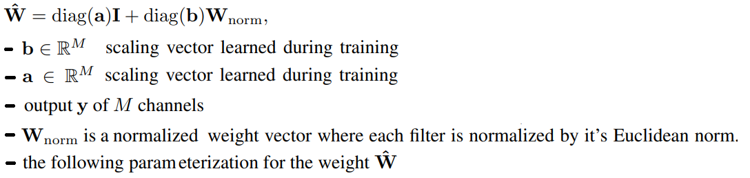
re-parameterization technique를 사용했다.favorable accuracy-speed trade-off 를 가진 모델이다.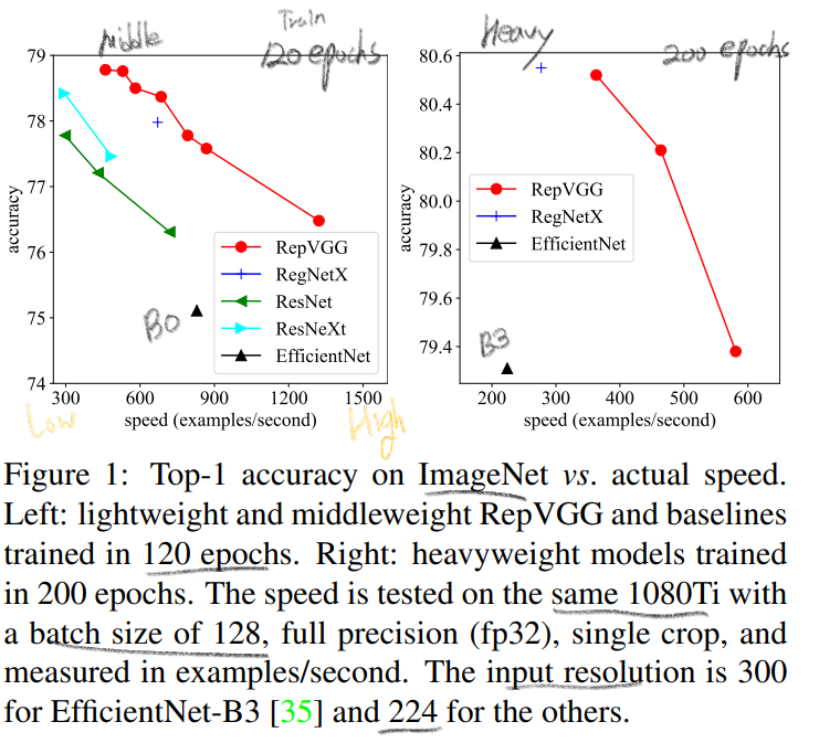
PS. 여기서, full precision(fp32): half precision이 fp16(floating point)을 Training 과정에서 효율적으로 사용하고 fp32도 중간중간에 사용하는 것이라면, full precision은 항상 fp32만 사용하는 것.
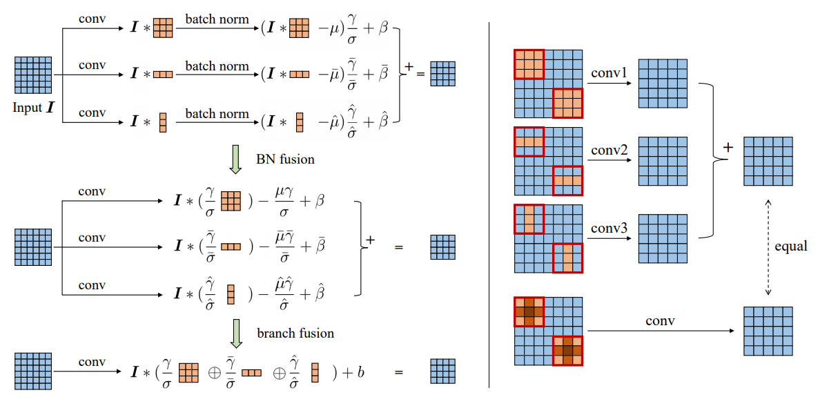
complicated ConvNets : Inception, ResNet, DensNet, EfficientNetdrawbackscomplicated multi-branch designs (ex, residual addition, branch-concatenation in Inception): 구현하기가 어렵다. Inference하는데 느리다. 메모리 사용을 더 많이 한다.without any branch 모델이다. 하지만 multi-branch 들과 유사한 성능을 내기에는 매우 challenging했다.avoids the gradient vanishing problem을 위해서 residual Block을 사용한다. 하지만! 이 모듈은 Inference 에서 필요가 없다.하기 위해서 re-parameterization` 사용했다. 전체 구조를 미리 대강 살펴보면 아래와 같다.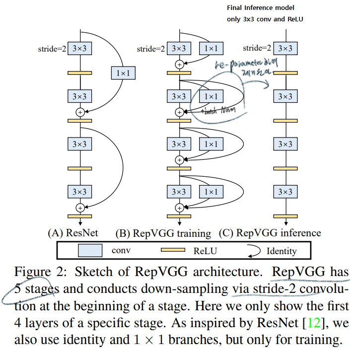
아래에 4.2 내용 참조
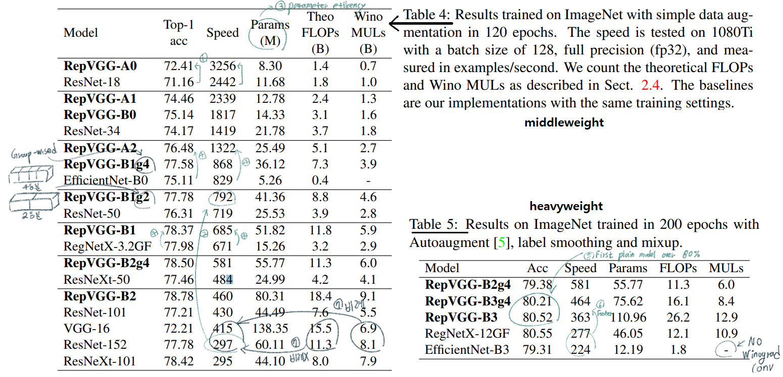
Winograd Algorithm을 사용하면 3x3 conv연산을 더욱 가속할 수 있다. Original 3x3 conv연산보다 the amount of multiplications (MULs)의 양이 4/9로 줄어든다. 우리는 이 알고리즘을 통한 연산을 딥러닝 프레임워크에서 default로 사용하고 있다.Tera FLoating-point Operations Per Second GPU 제작사에서 사용하는 지표로써 actual running time and computational density의 정도를 의미한다. 높을수록 좋다.time-consuming이 필요하기 때문이다.)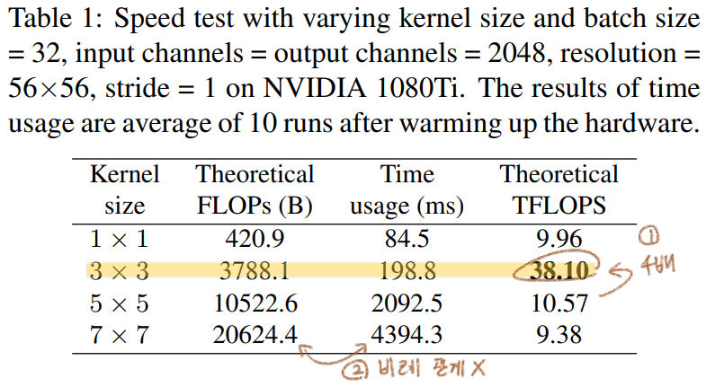
computational density가 대략 15배 차이 난다는 것을 의미한다.the memory access cost (MAC) (2) ` degree of parallelism ` 때문이다.MAC는 다른 연산에 비해서 높은 time-consuming이 필요하고, degree of parallelism이 높으면 빠른 연산이 가능하다.MAC가 거의 없고, parallelism이 매우 높다.NASNET-A(the number of individual conv or pooling operations in one building block): few (paralleism을 사용한) large operators이 아닌 multiple small operators을 사용하는 정도를 의미한다. 높을 수록 degree of parallelism이 안 좋은 것이다.multi-branch topology들은 memory-inefficient 하다. 예시는 아래의 그림에 있다.multi-branch topology에는 몇가지 제약이 있다.channel pruning to remove some unimportant channels 사용하지 못한다. (channel pruning)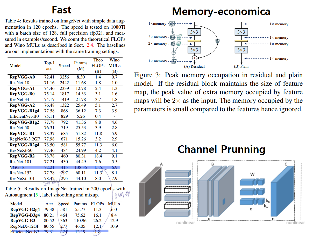
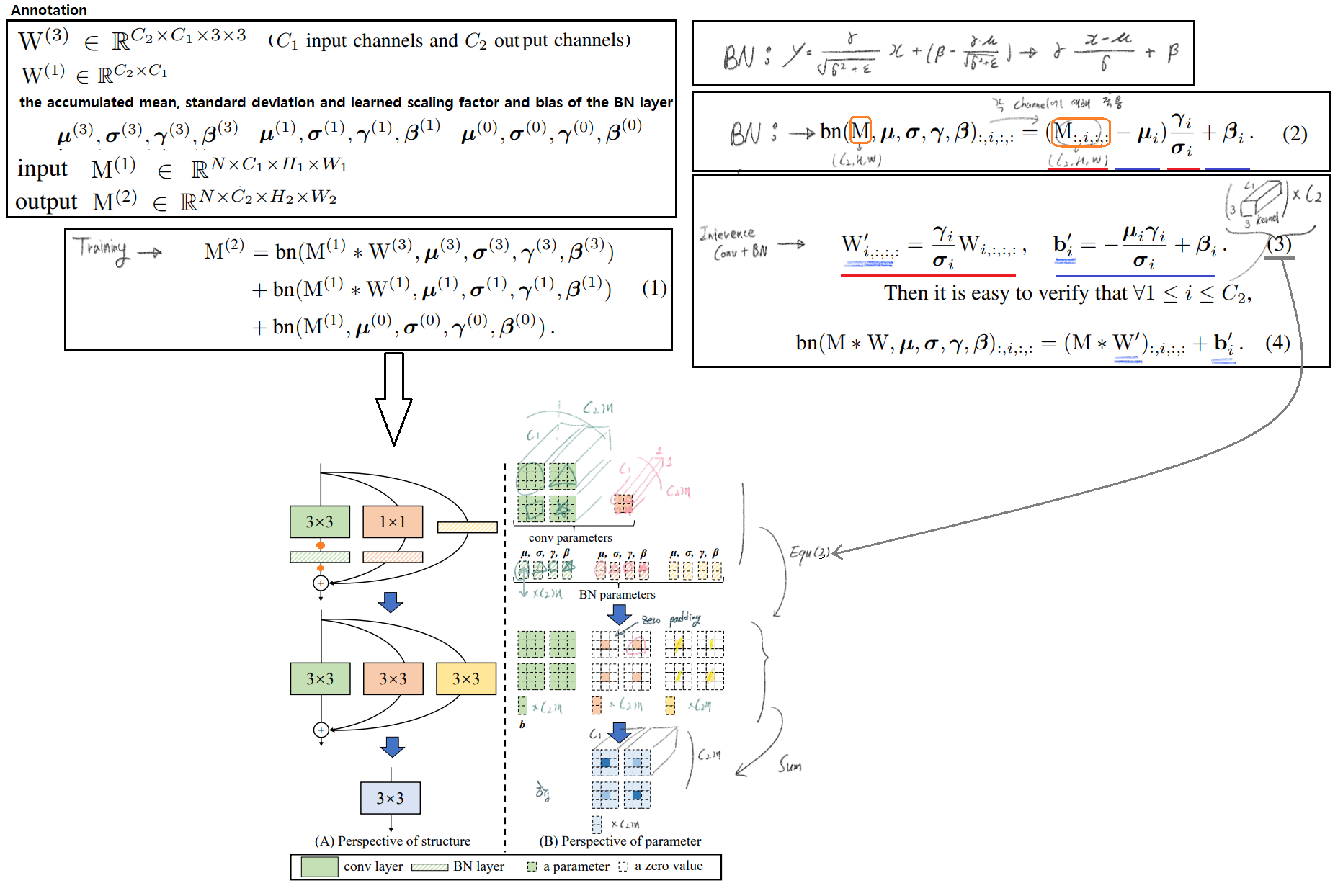
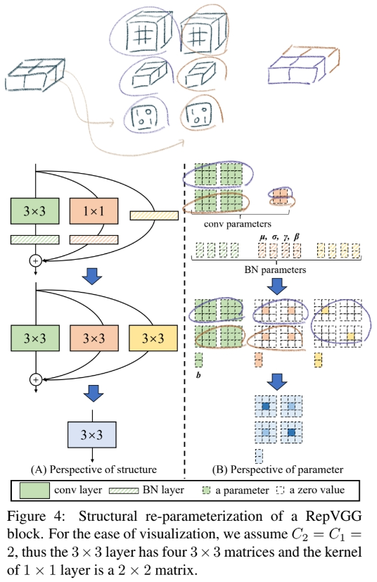
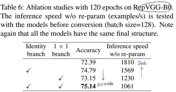
Residual block에 의해서 implicit (sum) ensemble model이라고 할 수 있다. n개의 block은 an ensemble of 2^n models이라고 표현가능하다. RepVGG는 an ensemble of 3^n models 모델을 만들었다. 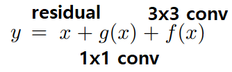
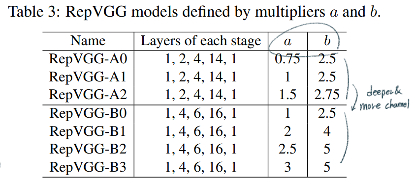
max pooling를 사용하지만, RepVGG에서는 최소한의 Operator만을 사용하기 위해서 사용하지 않는다.Global average pooling -> fully connected layerguidelines을 따라서 아래와 같은 Architecture models을 만들었다. 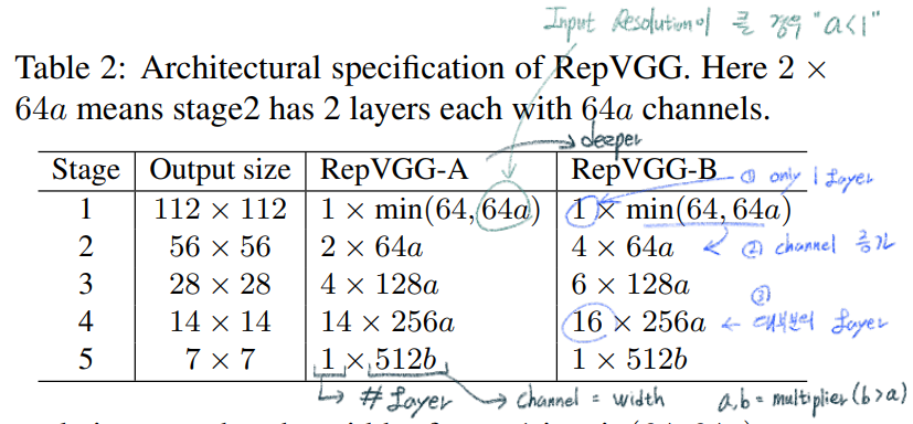
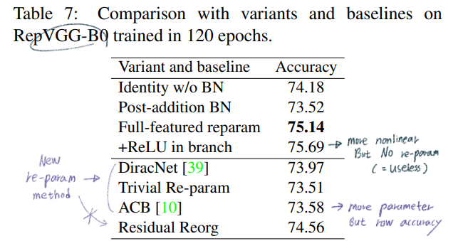
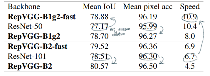
dilated conv를 적용한다. RepVGG에서도 dilated conv 구현하였지만, 속도가 많이 줄어들었다. (5*5로 padding한 conv를 사용해야하기 때문?)dilated conv를 적용한 것이 fast 모델이다.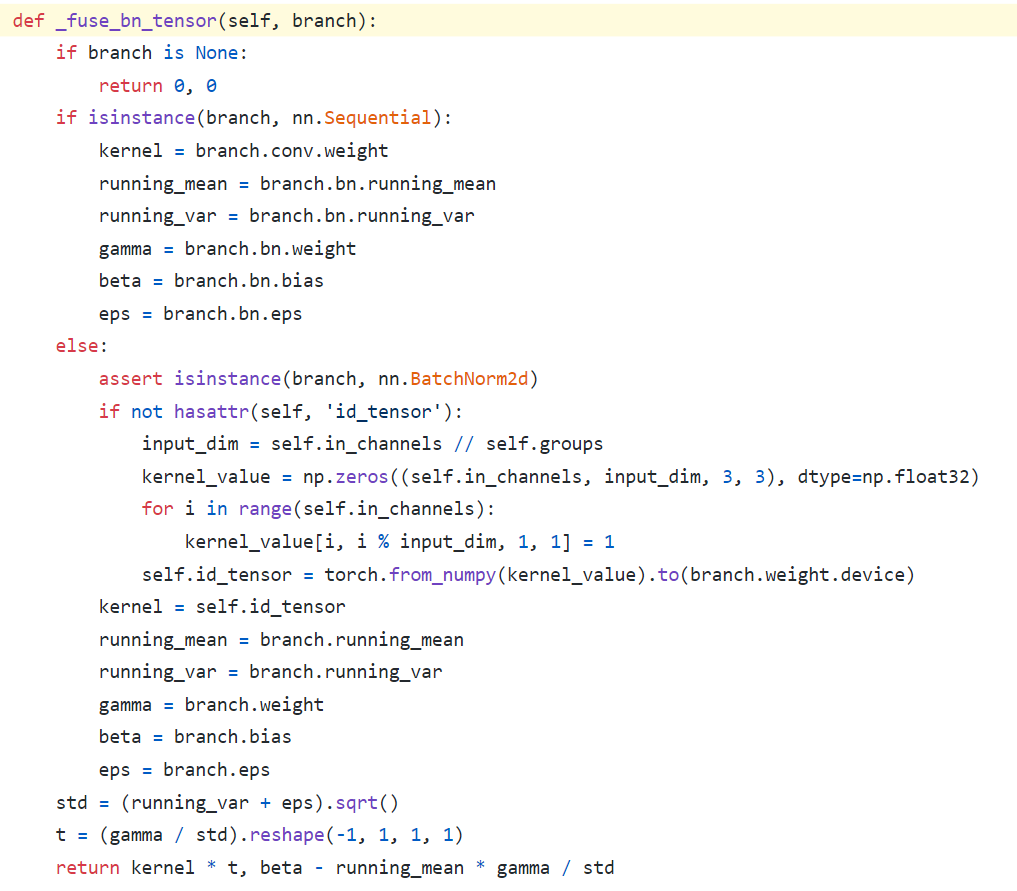
kernel_value = np.zeros((self.in_channels, input_dim, 3, 3), dtype=np.float32)에서 self.in_channels가 self.out_channels이 아닌 이유는, Skip_connection 연산은 input, output channel이 같기 때문이다.kernel_value[i, i % input_dim, 1, 1] = 1 코드가 위의 나의 그림 중 노란색으로 수정한 코드부분이다.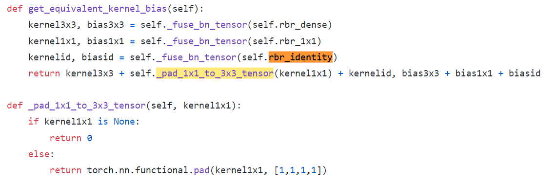
In this short guide, you’ll see how to Visualize torch.tensor or numpy.ndarray
how to Visualize torch.tensor or numpy.ndarray
# from via import via; via(x)
import numpy as np
import torch
import matplotlib
import matplotlib.pyplot as plt
import matplotlib.gridspec as gridspec

def via(arr, save_txt:bool = True, size:tuple = (20,20),
                out:str = 'array_out.txt', Normalize:bool = False):
    dim = arr.ndim
    if isinstance(arr, np.ndarray):
        # (#Images, #Chennels, #Row, #Column)
        if dim == 4:
            arr = arr.transpose(3,2,0,1)
        if dim == 3:
            arr = arr.transpose(2,0,1)
    if isinstance(arr, torch.Tensor):
        arr = arr.numpy()
    fig = plt.figure(figsize=size)

    if save_txt:
        with open(out, 'w') as outfile:
            outfile.write('# Array shape: {0}\n'.format(arr.shape))

            if dim == 1 or dim == 2:
                np.savetxt(outfile, arr, fmt='%-7.3f')

            elif dim == 3:
                for i, arr2d in enumerate(arr):
                    outfile.write('# {0}-th channel\n'.format(i))
                    np.savetxt(outfile, arr2d, fmt='%-7.3f')

            elif dim == 4:
                for j, arr3d in enumerate(arr):
                    outfile.write('\n\n# {0}-th Image\n'.format(j))
                    for i, arr2d in enumerate(arr3d):
                        outfile.write('# {0}-th channel\n'.format(i))
                        np.savetxt(outfile, arr2d, fmt='%-7.3f')
            else:
                print("Out of dimension!")


    if Normalize:
        arr -= np.min(arr)
        arr /= max(np.max(arr),10e-7)
    if dim == 1 or dim == 2:
        if dim==1: arr = arr.reshape((1,-1))
        fig.suptitle('Array shape: {0}\n'.format(arr.shape), fontsize=30)
        plt.imshow(arr, cmap='jet')
        plt.colorbar()
        plt.savefig('array_out.png')

    elif dim == 3:
        x_n = int(np.ceil(np.sqrt(arr.shape[0])))
        fig.suptitle('Array shape: {0}\n'.format(arr.shape), fontsize=30)
        for i, arr2d in enumerate(arr):
            ax = fig.add_subplot(x_n,x_n,i+1)
            im = ax.imshow(arr2d, cmap='jet')
            plt.colorbar(im)
            ax.set_title('{0}-channel'.format(i))
        fig.savefig('array_out.png')

    elif dim == 4:
        img_n = arr.shape[0]
        x_n = int(np.ceil(np.sqrt(arr.shape[1])))
        outer = gridspec.GridSpec(img_n, 1)
        fig.suptitle('Array shape: {0}\n'.format(arr.shape), fontsize=30)
        for j, arr3d in enumerate(arr):
            inner = gridspec.GridSpecFromSubplotSpec(x_n, x_n, subplot_spec=outer[j],wspace=0.1,hspace=0.3)
            for i, arr2d in enumerate(arr3d):
                ax = plt.subplot(inner[i])
                im = ax.imshow(arr2d, cmap='jet')
                plt.colorbar(im)
                ax.set_title('{0}-Image {1}-channel'.format(j,i))

        fig.suptitle('Array shape: {0}\n'.format(arr.shape), fontsize=30)
        fig.savefig('array_out.png')

    else:
        print("Out of dimension!")


arr = torch.rand(2,28,35)
via(arr, size=(20,20))
from pythonfile import Visualarr; Visualarr(x)
“The effect of initialization and architecture”, NIPS 2018 논문 내용을 사용했다.Distillation token : Class token과 같은 역할을 한다. 하지만, the (hard) label predicted by the teacher 만으로 학습된다. (Its target objective is given by the distillation component of the loss) = 아래 loss함수의 (Fun) + (Fun)에서 오른쪽 항 만을 사용해서 학습시킨다.
Distillation token으로 만들어 지는 Distillation Embeding의 결과도 Classfication Prediction 결과가 나와야 하는데, Teacher모델이 예측하는 결과가 나오면 된다. (이미지 자체 Label에 대해서는 학습되지 않는다.)

-01.png?raw=true)
-02.png?raw=true)
-03.png?raw=true)
-04.png?raw=true)
-05.png?raw=true)
-06.png?raw=true)
-07.png?raw=true)
-08.png?raw=true)
-09.png?raw=true)
-10.png?raw=true)
-11.png?raw=true)
-12.png?raw=true)
-13.png?raw=true)
-14.png?raw=true)
-15.png?raw=true)
-16.png?raw=true)
-17.png?raw=true)
-18.png?raw=true)
-19.png?raw=true)
-20.png?raw=true)
-21.png?raw=true)
-22.png?raw=true)
-23.png?raw=true)
-24.png?raw=true)
-25.png?raw=true)
-26.png?raw=true)
-27.png?raw=true)
-28.png?raw=true)
-29.png?raw=true)
-30.png?raw=true)
-31.png?raw=true)
-32.png?raw=true)