【RepVGG】 RepVGG- Making VGG style ConvNets Great Again
- 논문 : RepVGG: Making VGG-style ConvNets Great Again
분류 : ConNet
- 발표 위한 추가 정리 링크 : https://www.notion.so/RepVGG-717f8f09af6146e5bcd402c247337d29
RepVGG
0. Abstract
- 3 × 3 convolution와 ReLU 만을 사용하였다.
- Training과 Inference과정의 Architecture를 decoupling하였다. 이를 위해서 Training parameter를 VGG구조로 바꾸기 위한
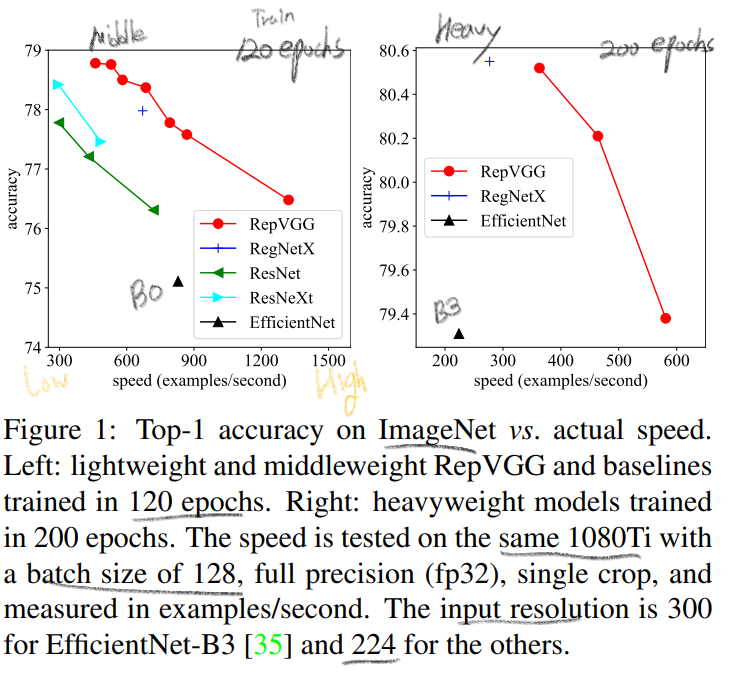
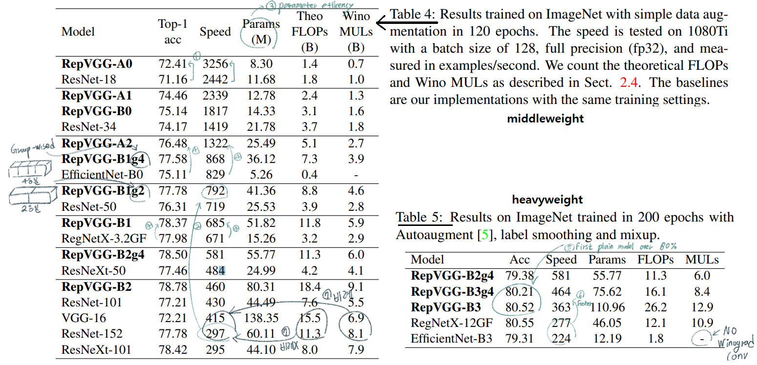
re-parameterization technique를 사용했다. - RepVGG의 결과 : (1080Ti) 80% top1 accuracy. (plain model에서는 최초로) ResNet보다 83% 빠르고, ResNet 101보다 101% 빠르다.
favorable accuracy-speed trade-off를 가진 모델이다.
PS. 여기서, full precision(fp32): half precision이 fp16(floating point)을 Training 과정에서 효율적으로 사용하고 fp32도 중간중간에 사용하는 것이라면, full precision은 항상 fp32만 사용하는 것.
1. Instruction
- 과거의 유명한 Backbone들
complicated ConvNets: Inception, ResNet, DensNet, EfficientNet - 이런 모델들의
drawbackscomplicated multi-branch designs(ex, residual addition, branch-concatenation in Inception): 구현하기가 어렵다. Inference하는데 느리다. 메모리 사용을 더 많이 한다.- depthwise conv(inverted residual), channel shuffle: various devices에서의 사용이 힘들다.
- 이 모델들의 FLOP(floating-point operations)과 Inference speed가 비례하지 않는다.
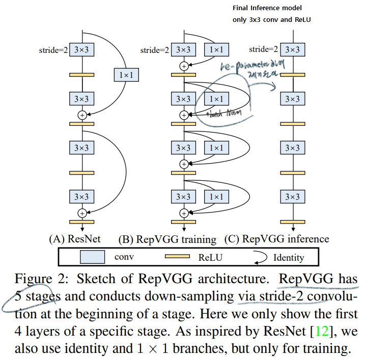
- 반면에 RepVGG는 VGG 같은 plain
without any branch모델이다. 하지만multi-branch들과 유사한 성능을 내기에는 매우 challenging했다. - ResNet의 장점이자 단점:
avoids the gradient vanishing problem을 위해서residual Block을 사용한다. 하지만! 이 모듈은 Inference 에서 필요가 없다. - 반면에 RepVGG는 Training과 Inference를 decouple했다. Training때 학습한 파라미터를 Inference모델로 ` equivalently replace
하기 위해서re-parameterization` 사용했다. 전체 구조를 미리 대강 살펴보면 아래와 같다. - Only 3x3 conv and ReLU로 구성되어 있기 때문에 빠르다. 만약 하나의 유닛이 fewer operator만을 수행한다면, 더 많은 computing 유닛을 가진 GPU를 만들어 낼 수 있다. 만약 3x3-Relu만을 수행하는 GPU가 존재한다면, 엄청난 수의 Unit을 가진 GPU가 될 것이다. 이 GPU에 특화될 수 있다. (특별한 GPU만들 수 있다면 RepVGG는 개꿀 모델이다.)
- Contributions
- favorable speed-accuracy trade-off
- re-parameterization
- effectiveness at classification and sementic segmentation
2. Related Work
2.3. Model Re-parameterization
아래에 4.2 내용 참조
2.4 Winograd Convolution
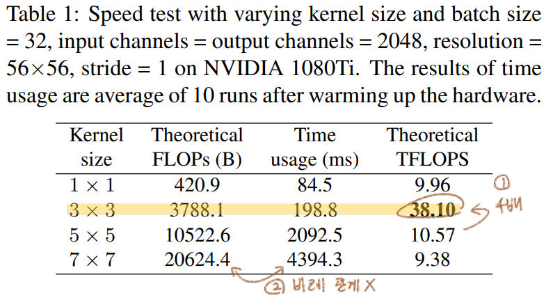
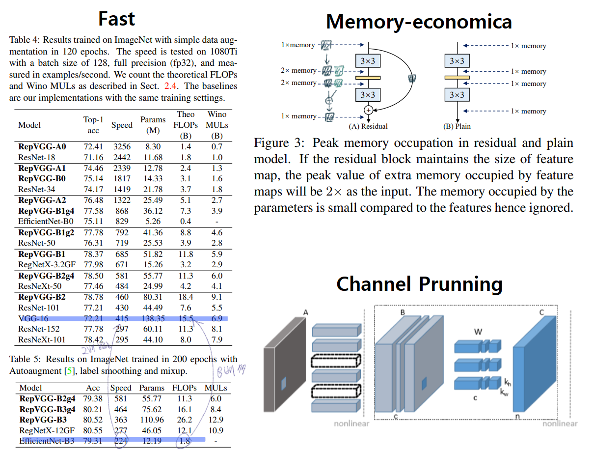
- RepVGG는 only 3x3 conv로만 구성되어 있는데, GPU라이브러리는 이 연산에 매우 최적화 되어있다. 위의 표에서 주목해야할 점을 기록해 놓았다.
Winograd Algorithm을 사용하면 3x3 conv연산을 더욱 가속할 수 있다. Original 3x3 conv연산보다the amount of multiplications (MULs)의 양이 4/9로 줄어든다. 우리는 이 알고리즘을 통한 연산을 딥러닝 프레임워크에서 default로 사용하고 있다.- TFLOPS:
Tera FLoating-point Operations Per SecondGPU 제작사에서 사용하는 지표로써 actual running time and computational density의 정도를 의미한다. 높을수록 좋다. - (Table4,5에서 MULs을 기준으로 한 비교를 할 예정이다. Additions연산보다 multiplication연산이 더 많은
time-consuming이 필요하기 때문이다.)
3. Building RepVGG
3.1. simple ConvNets의 장점
- Fast
- FLOP과 Speed는 비례하지 않는다. 아래의 비교를 보면 VGG16이 FLOPs가 8배 높지만, 2배 빠르다. 즉
computational density가 대략 15배 차이 난다는 것을 의미한다. - Simple Conv는 FLOP이 높아도 Speed는 훨씬 빠르다. 그 이유는 (1)
the memory access cost (MAC)(2) ` degree of parallelism ` 때문이다. MAC는 다른 연산에 비해서 높은time-consuming이 필요하고,degree of parallelism이 높으면 빠른 연산이 가능하다.- plain conv는
MAC가 거의 없고,parallelism이 매우 높다. NASNET-A(the number of individual conv or pooling operations in one building block):few (paralleism을 사용한) large operators이 아닌multiple small operators을 사용하는 정도를 의미한다. 높을 수록degree of parallelism이 안 좋은 것이다.
- FLOP과 Speed는 비례하지 않는다. 아래의 비교를 보면 VGG16이 FLOPs가 8배 높지만, 2배 빠르다. 즉
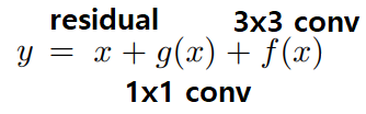
- Memory-economica
multi-branch topology들은 memory-inefficient 하다. 예시는 아래의 그림에 있다.
- Flexible
multi-branch topology에는 몇가지 제약이 있다.- 제약1: the last conv layers of every residual block have to produce tensors of the same shape
- 제약2 :
channel pruningto remove some unimportant channels 사용하지 못한다. (channel pruning)
- 반면에 RepVGG는 자유로는 shape 구성이 가능하고, channel pruning 또한 가능하다.
3.2 Training-time Multi-branch Architecture
- Plain conv = the poor performance. 따라서 Training과정에서는 multi-branch 모델의 장점을 최대한 이용한다.
- ResNet의
Residual block에 의해서implicit (sum) ensemble model이라고 할 수 있다. n개의 block은an ensemble of 2^n models이라고 표현가능하다. RepVGG는an ensemble of 3^n models모델을 만들었다.
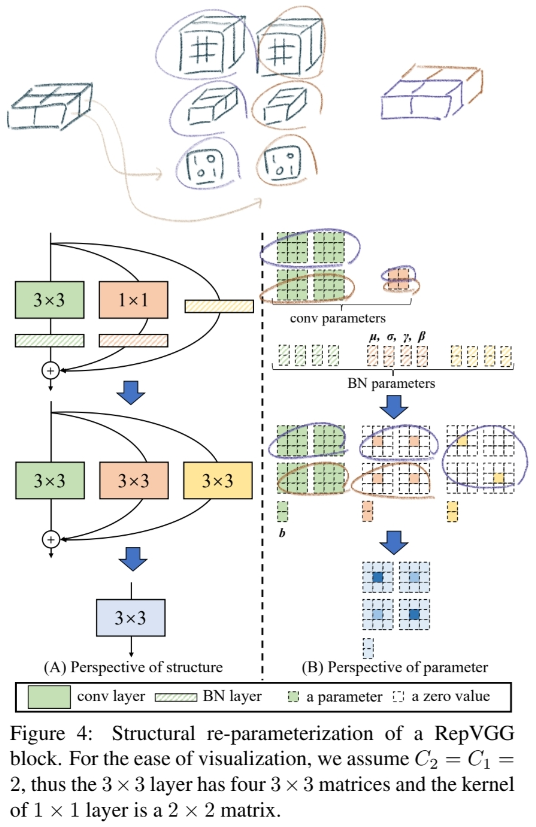
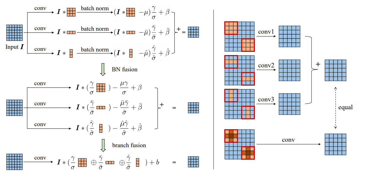
3.3. Re-param for Plain Inference-time Model
- 코드를 바탕으로 제대로 다시 제대로 그려놓은 그림
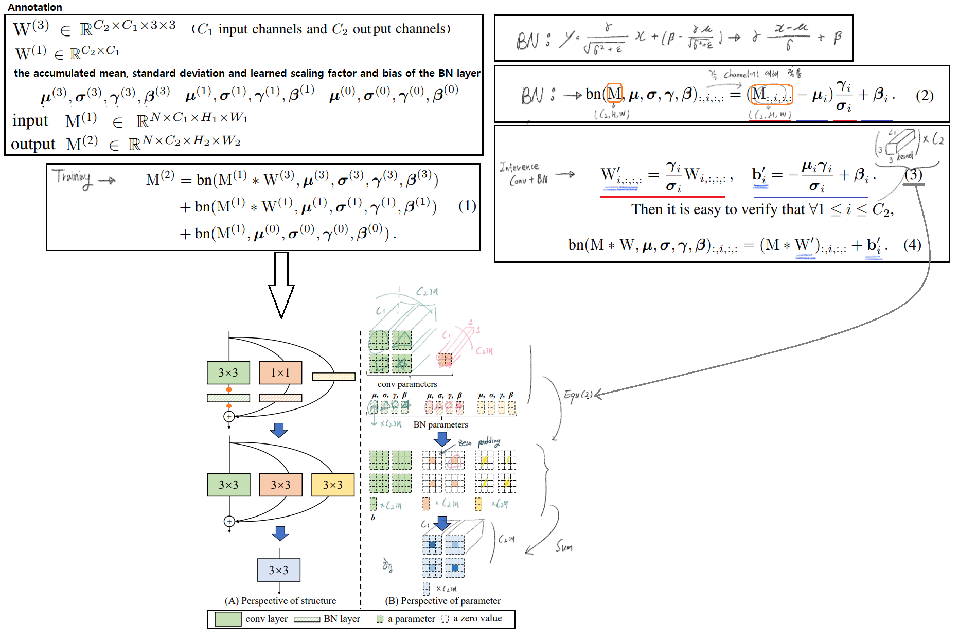
- 하지만 굳이 논문 내용으로 이해하고 싶다면, 아래와 같이 해석할 수 있다.
- (한 채널의 2차원 평면을 단위 행렬을 곱하여, 똑같은 2차원 평면이 나오게 만든다.)
3.4. Architectural Specification
- VGG에서는
max pooling를 사용하지만, RepVGG에서는 최소한의 Operator만을 사용하기 위해서 사용하지 않는다. - 5 stage, the first layer of stage with stride=2
- classification위해서 RepVGG를 통과한 후,
Global average pooling -> fully connected layer - 몇가지
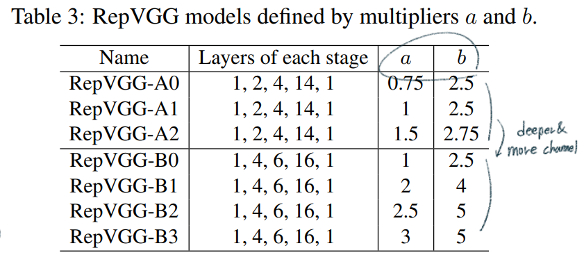
guidelines을 따라서 아래와 같은 Architecture models을 만들었다.
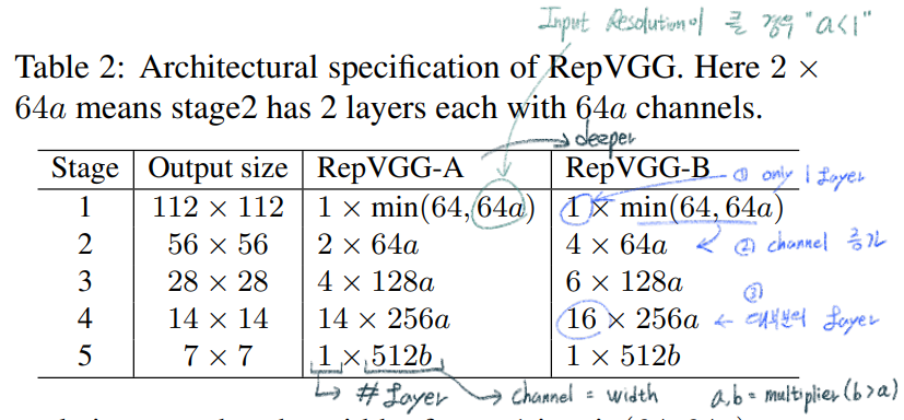
- 특별히 b를 사용하는 이유는, 5 stage에 어차피 1개의 layer만을 사용하니, channel을 최대한으로 늘려도 모델 전체 파라미터 양에 큰 영향을 주지 않으므로 b를 사용한다.
- further 파라미터를 줄이기 위해서, Groupwise conv layer를 사용한다.
- 3rd, 5th, 7th, …, 21st layer of RepVGG-A
- 3rd, 5th, 7th, …, 21st, 23rd, 25th and 27th layers of RepVGG-B
- (channel을 몇등분으로 나눌지) g = 1 or 2 or 4
4. Experiments
4.1. RepVGG for ImageNet Classification
- data augmentation: random cropping and left-right flipping
- batch size of 256 on 8 GPUs
- 위의 Architecture에서 a와 b를 다르게 설정하여, middleweight and heavyweight models을 만들어 낸다.
4.2. Structural Re-parameterization is the Key
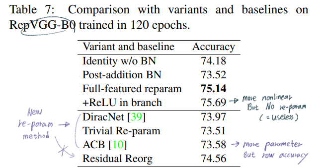
- Ablation studies
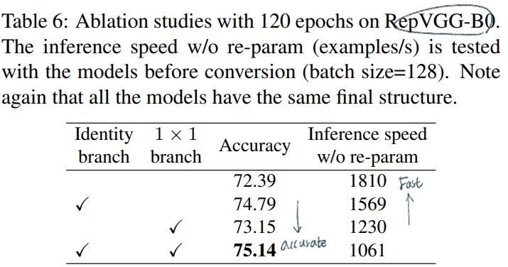
- Re-parameterizaition 성능 비교: 각각에 대한 자세한 설명은 논문에서 잘 분류해 놓았으니 참고
- 추가 실험
- ResNet50에서 모든 3x3 conv를 RepVGG block으로 바꾸고 학습시킨 후 re-parameterization을 통해서 다시 simple 3x3 conv로 바꿨을 때, 성능이 0.03% 상승해다. -> 강력한 plain convNet을 학습시키기 위해, 우리의 방법이 매우 유용하다!
- RepVGG에 추가적인 Skip-connection을 추가했을때, 성능이 0.58% 상승하였다. residual로써 ensemble 모델이 내제적으로 구현된 것이기 때문에 당연하다.
- 보충 설명
- DiracNet
- 비슷하면서 조금 다른 모듈이다.
- RepVGG에서는 scaling vector 없음, BN 고려, Bias 고려, 1x1 conv 추가
- 논문에서 이야기 하는 차이점
- RepVGG는 actual dataflow through a concrete structure 를 따른다. 반면에 DiracNet은 easier optimization를 위해서 ` another mathematical expression of conv kernels`을 사용했을 뿐이다.
- 성능이 RepVGG보다, 다른 SOTA 모델보다 떨어진다.
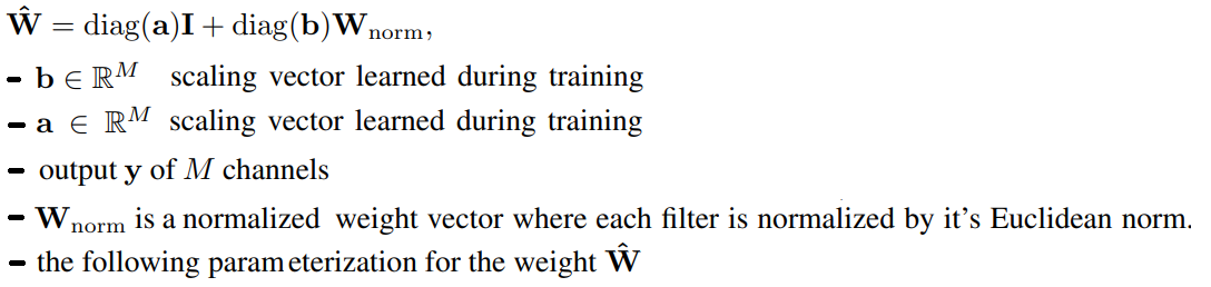
- Trivial Re-param
- 위의 식에서 a = 1,b = 1
- ACB
- 아래와 같이 3x3 conv를 more parameter를 사용하는 conv로 바꿔서 학습시킨다. 그리고 다시 3x3conv를 아래와 같이 변환한다.
- 아래와 같이 3x3 conv를 more parameter를 사용하는 conv로 바꿔서 학습시킨다. 그리고 다시 3x3conv를 아래와 같이 변환한다.
- DiracNet
4.3. Semantic Segmentation
- ImageNetpretrained RepVGG 사용했다
- PSPNet 사용
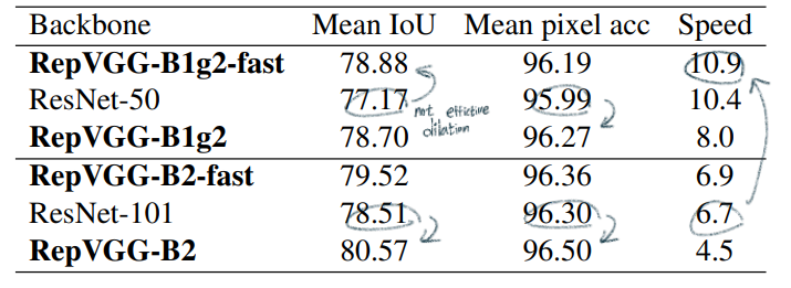
- PSPNet는 stage 3,4에서
dilated conv를 적용한다. RepVGG에서도dilated conv구현하였지만, 속도가 많이 줄어들었다. (5*5로 padding한 conv를 사용해야하기 때문?) - 그래서 last 5 layers에서만
dilated conv를 적용한 것이 fast 모델이다. - 결과 분석
- ResNet101과 성능이 비슷한 RepVGG-B1g2-fast의 속도가 62%나 빠르다.
- middleweight 모델에서는 dilation이 그리 효율적이지 않다.
4.4 Limitation
- RepVGG models은 단순 연산을 하는 unit이 많은 GPU에 매우 효율적이다.
- 하지만 GPU가 없는 mobile-regime에서는 효율적은 모델은 아니다.
- CPU를 위한 모델 -> MobileNet // low-power -> ShuffleNet (연산량이 매우 적다)
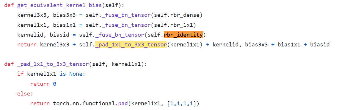
Code
- Equation (3): 여기서 else가 Identity(only nn.BatchNorm2d) To W’+b’로 변환하는 코드이다.
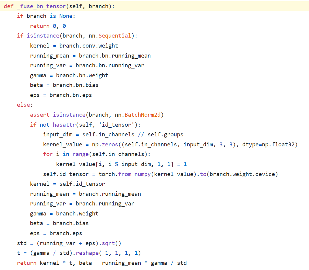
kernel_value = np.zeros((self.in_channels, input_dim, 3, 3), dtype=np.float32)에서self.in_channels가self.out_channels이 아닌 이유는, Skip_connection 연산은 input, output channel이 같기 때문이다.- 특히
kernel_value[i, i % input_dim, 1, 1] = 1코드가 위의 나의 그림 중 노란색으로 수정한 코드부분이다.
- Sum