# 예제코드
from__future__importprint_functionimportargparsedefmain():parser=argparse.ArgumentParser(description='This code is written for practice about argparse')parser.add_argument('X',type=float,metavar='First_number',help='What is the first number?')parser.add_argument('Y',type=float,metavar='Second_number',help='What is the second number?')parser.add_argument('--op',type=str,default='add',choices=['add','sub','mul','div'],help='What operation?')args=parser.parse_args()X=args.XY=args.Yop=args.opprint(calc(X,Y,op))defcalc(x,y,op):ifop=='add':returnx+yelifop=='sub':returnx-yelifop=='mul':returnx*yelifop=='div':returnx/yif__name__=="__main__":main()
기초 코드
argparse.ArgumentParser함수를 통해 parser를 생성한다.
parser.add_argument를 이용하여 입력받고자 하는 인자의 조건을 설정한다
parser.parse_args 함수를 통해 인자들을 파싱하여 args에 저장한다. 각 인자는 add_argument의 type에 지정된 형식으로 저장된다
parser.add_argument에 들어갈 수 있는 옵션
type/ default/ choices/ help 등등
여기서 choices를 사용함으로써 help에서 어떤 옵션이 가능한지 보여준다.
metavar는 필수 인자를 입력하지 않았을 때, 그 자리 변수가 무엇인지에 대한 이름이다.
nargs=’+’를 사용함으로써, 여러개의 (제한 없음) 변수를 리스트로 받을 수 있다.
parser.parse_args()로 정의된 객체 args 사용방법
X = args.X // Y = args.Y
op = args.op 에서 처럼 –[]라고 add_argument를 했다면, args.[]라고 사용가능하다.
두번쨰 Reference 공부내용 정리
위의 기초 코드 3개 중, ArgumentParser와 add_argument에 사용가능한 메소드들이 잘 정리되어 있다.
즉, yaml 모듈의 load함수를 통해서 conf를 dictionary 객체로 만들어 준다.
추가 사용법
모르겠으면 우선 yaml파일을 가져오고, type과 같은 함수를 이용해서 내가 가지고 있는 yaml.load로 선언한 객체에 대한 분석을 해보자.
코드 예제
# yaml 파일
yaml_str="""
Date: 2017-08-08
ChampionList:
- champion_id: 1000
name: Teemo
position: top
skill: ap
- champion_id: 1001
name: Vayne
position: bottom
skill: ad
- champion_id: 1002
name: Ahri
position: mid
skill: ap
"""# .py 파일 내부 코드
importyamlcfg=yaml.load(yaml_str)forchampionincfg['ChampionList']:print(champion["name"],champion["skill"])
로그 출력을 위한 logging 모듈을 제공합니다. 아주 간단히 사용할 수 있으며, print 함수 등을 통해 콘솔창에 지저분하게 출력하는 것보다 logging 모듈을 사용하는 것을 추천한다. 콘솔창과 파일에 동시에 로그 남기는 것이 가능하다.
로그를 콘솔에도 출력하고 싶고, 파일에도 동시에 남기고 싶다면 아래와 같이 fileHandler, streamHandler를 생성해서 logger에 Handler를 추가해주면 된다
로그 포매팅이라고 하면, 내가 로그를 남길때 앞에 쓰여지는 형식의 포맷을 정하는 것을 말한다 로그 포매팅 : %(log_name)s 를 사용하고 중간에 문자를 자유롭게 첨가
importloggingimportlogging.handlers# logger 인스턴스를 생성 및 로그 레벨 설정
logger=logging.getLogger("crumbs")logger.setLevel(logging.DEBUG)# formmater 생성 <***adding***>
formatter=logging.Formatter('[%(levelname)s|%(filename)s:%(lineno)s] %(asctime)s > %(message)s')# fileHandler와 StreamHandler를 생성
fileHandler=logging.FileHandler('./log/my.log')streamHandler=logging.StreamHandler()# handler에 fommater 세팅 <***adding***>
fileHandler.setFormatter(formatter)streamHandler.setFormatter(formatter)# Handler를 logging에 추가
logger.addHandler(fileHandler)logger.addHandler(streamHandler)# logging
logger.debug("debug")logger.info("info")logger.warning("warning")logger.error("error")logger.critical("critical")'''
출력결과
[DEBUG|input.py:24] 2016-05-20 10:37:06,656 > debug
[INFO|input.py:25] 2016-05-20 10:37:06,657 > info
[WARNING|input.py:26] 2016-05-20 10:37:06,657 > warning
[ERROR|input.py:27] 2016-05-20 10:37:06,657 > error
[CRITICAL|input.py:28] 2016-05-20 10:37:06,657 > critical
다른 코드를 통해 좀 더 알아보자. setLevel(logging.DEBUG) -> setLevel(logging.INFO)
importlogging# 로그 생성
logger=logging.getLogger()# 로그의 출력 기준 설정
logger.setLevel(logging.INFO)# log 출력 형식 기본 포맷
formatter=logging.Formatter('%(asctime)s - %(name)s - %(levelname)s - %(message)s')# log 출력
stream_handler=logging.StreamHandler()stream_handler.setFormatter(formatter)logger.addHandler(stream_handler)# log를 파일에 출력
file_handler=logging.FileHandler('my.log')file_handler.setFormatter(formatter)logger.addHandler(file_handler)foriinrange(10):logger.info(f'{i}번째 방문입니다.')ㄴ
이 논문에서는 deep learning이 무엇이고 CNN이 무엇인지에 대한 아주 기초적인 내용들이 들어가 있다. 이미 알고 있는 내용들이라면 매우 쉬운 논문이라고 할 수 있다.
FCN에 대한 소개를 해주고, a virtual city Image인 SYNTHIA-Rand-CVPR16 Dataset을 사용해, FCN-AlexNet, FCN-8s, FCN-16s and FCN-32s 이렇게 4가지 모델에 적용해 본다.
결론 :
Maximum validation accuracies of 92.4628%, 96.015%, 95.4111% and 94.2595% are achieved with FCN-AlexNet, FCN-8s, FCN-16 and FCN-32s models
Training times는 FCN-AlexNet이 다른 모델들에 비해 1/4시간이 걸릴 만큼 학습시간이 매우 짧다. 하지만 우리에게 중요한 것은 inference시간이므로, the most suitable model for the application is FCN-8s.
ParsNet – Global context information, Global pooling,
SegNet – Encoder/Decoder, maxpooling index
HRNet – high resolution, low resolution의 information Exchange. BackboneNetwork
Panotic-Network (PA-Net) – FPN + mask+rcnn
Dilated Conv – 추가 비용없이, receptive field 확장
RNN, LSTM, Attention, GAN 개념 사용 가능
CRF – Posterior를 최대화하고 Energy를 최소화한다. Energy는 위치가 비슷하고 RGB가 비슷한 노드사이에서 라벨이 서로 다른것이라고 하면 Panalty를 부과함으로써 객체의 Boundary를 더 정확하게 찾으려고 하는 노력입니다. Energy공식에 비용이 너무 많이 들어서 하는 작업이 mean field approximation이라고 합니다.
Yolo – 1stage detector, cheaper grid, 7730(5+5+20), confidence낮음버림, NMS -> Class 통합
SSD – Anchor, 다양한 크기 객체, 작은 -> 큰 물체, Detector&classifier(3개 Anchor, locallization(x,y,w,h), class-softMax결과(20+1(배경)) ), NMS
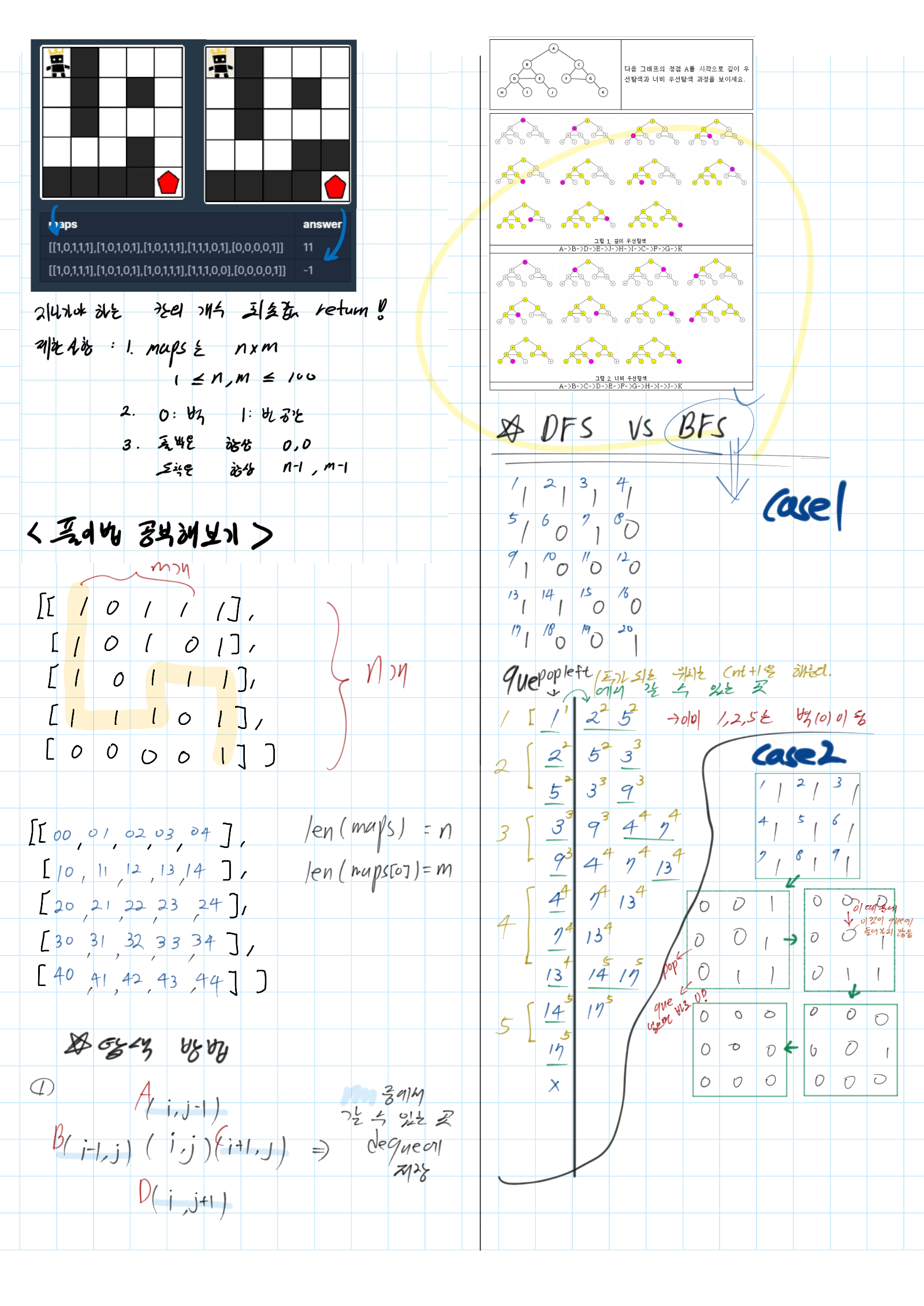
fromcollectionsimportdequedefbfs(start,maps):dirs=[(0,1),(1,0),(0,-1),(-1,0)]queue=deque()# https://excelsior-cjh.tistory.com/96
queue.append(start)whilequeue:# 빈 list, 빈 que는 False가 된다.
y,x,cnt=queue.popleft()maps[y][x]=0# Point! 이미 방문한 곳 처리는 벽으로 만들어 버린다!
fordy,dxindirs:ny,nx=y+dy,x+dx# BFS를 사용하므로, 가장 처음 발견하면, 그 cnt를 return하면 된다.
ifny==len(maps)-1andnx==len(maps[0])-1:returncnt+1# 빈 공간을 만났다면,
elif0<=ny<len(maps)and0<=nx<len(maps[0])andmaps[ny][nx]==1:maps[ny][nx]=0queue.append((ny,nx,cnt+1))return-1defsolution(maps):# 첫 위치는, map[0][0]이며, count=1로 시작한다.
returnbfs((0,0,1),maps)
점진적에서 하나 개의 기능을 추가 할 것 -> torch.nn, torch.optim, Dataset, DataLoader
처음에는 정말 코드를 복잡하게 만들고, 그것을 torch 내부의 모듈과 함수(클래스)를 이용해서 코드를 점점 쉽게 구현해 나갈 것이다.
1. 파일 및 이미지 다운. 파일을 torch.tensor로 변환하기
frompathlibimportPath# pathlib는 파일위치 찾기, 파일 입출력에 사용하는 모듈. 과거 os모듈. https://brownbears.tistory.com/415
importrequests# 간편한 HTTP 요청처리를 위해 사용하는 모듈
# 1. 폴더를 만들고, MNIST 데이터 다운로드 하기
DATA_PATH=Path("data")PATH=DATA_PATH/"mnist"# os.path.join 과 같은 느낌.
PATH.mkdir(parents=True,exist_ok=True)URL="http://deeplearning.net/data/mnist/"FILENAME="mnist.pkl.gz"ifnot(PATH/FILENAME).exists():# os.path.join 과 같은 느낌.
content=requests.get(URL+FILENAME).content(PATH/FILENAME).open("wb").write(content)# 2. 다운한 파일의 압축을 풀고, 파일을 Load 하여, 하나의 변수에 넣는다.
importpickle# 파일 load하는데 많이 쓰이는 모듈
importgzip# 압축된 파일의 내용을(굳이 압축안 풀고) 바로 읽을 수 있게 해주는 모듈 : https://itholic.github.io/python-gzip/
withgzip.open((PATH/FILENAME).as_posix(),"rb")asf:((x_train,y_train),(x_valid,y_valid),_)=pickle.load(f,encoding="latin-1")
# 3. 파일 다운로드가 잘 되었나 확인하보자.
frommatplotlibimportpyplotimportnumpyasnpprint(x_train.shape,'\n',type(x_train))pyplot.imshow(x_train[0].reshape((28,28)),cmap="gray")
(50000, 784)
 <class 'numpy.ndarray'>


<matplotlib.image.AxesImage at 0x2930e3d3088>
# 4. torch.tensor를 사용할 것이기 때문에,
importtorchx_train,y_train,x_valid,y_valid=map(torch.tensor,(x_train,y_train,x_valid,y_valid))# https://pytorch.org/docs/stable/tensors.html#torch.Tensor
n,c=x_train.shapeprint(x_train.shape)print(y_train.min(),y_train.max())# 0 ~ 9까지 10개의 Class가 존재한다.
torch.Size([50000, 784])
tensor(0) tensor(9)
2. torch.nn을 사용하지 않고 신경망 구현해 보기.
nn을 이용해서, 매개변수를 정의한다면, 자동으로 requires_grad = True가 된다. 하지만 아래와 같이 매개변수를 직접 정의한다면, requires_grad = True를 직접해주어야한다. 그리고, _를 사용하면 the operation is performed in-place라는 것을 의미한다.
importmathweights=torch.randn(784,10)/math.sqrt(784)# 여기서 가중치 초기화 방법으로 Xavier initialisation 를 사용했다.
weights.requires_grad_()# Defalut =-> requires_grad=True : https://pytorch.org/docs/stable/tensors.html#torch.Tensor.requires_grad_
bias=torch.zeros(10,requires_grad=True)
# 1층 Fully connected Layer를 만든다.
deflog_softmax(x):returnx.exp().log()-x.exp().sum(-1).log().unsqueeze(-1)# torch.tensor의 함수(math 모듈의 함수 NO)를 잘 이용하고 있다.
# x.exp().log() == x
defmodel(xb):returnlog_softmax(xb@weights+bias)# @내적 연산을 의미
# 64장을 하나의 배치로 하고, Forward를 진행해 나간다.
bs=64# batch size
xb=x_train[0:bs]# a mini-batch from x
preds=model(xb)# predictions
print(preds[0])print(preds.shape)
defnll_loss(input,target):return-input[range(target.shape[0]),target].mean()loss_func=nll_loss# 함수 포인터는 이처럼 이용하면 된다.
yb=y_train[0:bs]print(yb.shape)# torch.Size([64]) -> 64장의 이미지 각각의 class가 적혀 있다.
print(loss_func(preds,yb))
defaccuracy(preds_before,yb):# 각 예측에 대해 가장 큰 값을 가진 인덱스가 목표 값과 일치함을 판단합니다.
preds=torch.argmax(preds_before,dim=1)# dim : the dimension to reduce. If None, the argmax of the flattened input is returned.
# preds_before -> shape : (64, 10) -> (64)
return(preds==yb).float().mean()"""
print(preds) -> tensor([3, 3, 3, 6, 6, 3, 3..... 9, 3, 6])
print(preds.shape) -> torch.Size([64])
"""print(accuracy(preds,yb))
tensor(0.0312)
이제 훈련을 시켜보자.
loop를 통해서, 데이터 가져오기 -> forward -> loss계산 -> backward -> 가중치 갱신 이 되는 것을 확인하라.
fromIPython.core.debuggerimportset_tracelr=0.5# learning rate
epochs=2# how many epochs to train for
forepochinrange(epochs):# x_train.shape == (50000,784)
# n == 50000 , bs = 64
foriinrange((n-1)//bs+1):# set_trace()
# 튜토리얼 문서에 의하면, 이 코드를 디버깅하면서 한줄한줄 확인하고 싶다면 위의 주석을 풀라 했다.
start_i=i*bsend_i=start_i+bsxb=x_train[start_i:end_i]yb=y_train[start_i:end_i]pred=model(xb)loss=loss_func(pred,yb)loss.backward()withtorch.no_grad():weights-=weights.grad*lrbias-=bias.grad*lrweights.grad.zero_()bias.grad.zero_()# 여기서 x_train의 가장 마지막 16개의 사진은 학습에 사용 못 된다.
print(loss_func(model(xb),yb),"\n",accuracy(model(xb),yb))# 가장 마지막 배치에 대한, loss와 accuracy를 확인해보자
tensor(0.0827, grad_fn=<NegBackward>)
 tensor(1.)
3. Using torch.nn.functional
위에서 했던 동일한 작업을 수행하기 위해, PyTorch의 nn클래스를 활용하여보다 간결하고 유연한 코드를 만들어보자. 우선 torch.nn.functional를 사용해서 코드를 만들어 봅시다. 여기에는 torch.nn의 모든 기능이 포함되어 있습니다.
# 새로운 학습을 위해.. 다시!
xb=x_train[0:bs]# a mini-batch from x
yb=y_train[0:bs]weights=torch.randn(784,10)/math.sqrt(784)# 여기서 가중치 초기화 방법으로 Xavier initialisation 를 사용했다.
weights.requires_grad_()# Defalut =-> requires_grad=True : https://pytorch.org/docs/stable/tensors.html#torch.Tensor.requires_grad_
bias=torch.zeros(10,requires_grad=True)
importtorch.nn.functionalasFloss_func=F.cross_entropy# 위의 nll_loss 처럼, 함수 포인터는 이처럼 이용하면 된다.
defmodel(xb):returnxb@weights+biasprint(loss_func(model(xb),yb),accuracy(model(xb),yb))
fromtorchimportnn# import torch.nn as nn
classMnist_Logistic(nn.Module):def__init__(self):super().__init__()# nn.Parameter(텐서) : 이 텐서를 parameter로 이용할 것을 명명한다. grad를 알아서 해준다.
self.weights=nn.Parameter(torch.randn(784,10)/math.sqrt(784))self.bias=nn.Parameter(torch.zeros(10))defforward(self,xb):returnxb@self.weights+self.bias
# 위에서는 weights -= weights.grad * lr -> weights.grad.zero_() 과 같은 과정을 bias에도 반복했었지만.. 여기서는 쉽게 할 수 있다.
withtorch.no_grad():forpinmodel.parameters():p-=p.grad*lrmodel.zero_grad()
fromIPython.core.debuggerimportset_tracelr=0.5# learning rate
epochs=2# how many epochs to train for
deffit():forepochinrange(epochs):foriinrange((n-1)//bs+1):start_i=i*bsend_i=start_i+bsxb=x_train[start_i:end_i]yb=y_train[start_i:end_i]pred=model(xb)loss=loss_func(pred,yb)loss.backward()withtorch.no_grad():forpinmodel.parameters():p-=p.grad*lrmodel.zero_grad()fit()
print(loss_func(model(xb),yb))
5. Refactor using nn.Linear
위에서는 weight와 bias를 직접 정의했지만, 이제는 nn.Linear를 사용해서 코드를 구현해보자
fromtorchimportoptim# 더 아래에서도 사용하기 위해서, 굳이 이렇게 get_model이라는 함수를 구현했다.
defget_model():model=Mnist_Logistic()returnmodel,optim.SGD(model.parameters(),lr=lr)model,opt=get_model()"""
model = Mnist_Logistic()
opt = optim.SGD(model.parameters(), lr=lr)
"""print(loss_func(model(xb),yb))lr=0.5epochs=2forepochinrange(epochs):foriinrange((n-1)//bs+1):start_i=i*bsend_i=start_i+bsxb=x_train[start_i:end_i]yb=y_train[start_i:end_i]pred=model(xb)loss=loss_func(pred,yb)loss.backward()opt.step()opt.zero_grad()print(loss_func(model(xb),yb))
를 했지만, 파이토치의 an abstract Dataset class인, TensorDataset를 이용해보자. (텐서의 첫 번째 차원을 따라 반복, 인덱싱 및 슬라이스하는 방법을 제공) TensorDataset에는 len , getitem 이라는 좋은 함수가 있다. * 자세한 사항은 이 홈페이지를 공부하자 **언젠간 공부해야 한다!! ***
fromtorch.utils.dataimportTensorDatasettrain_ds=TensorDataset(x_train,y_train)""" 위에서는 이렇게 했었다.
start_i = i * bs
end_i = start_i + bs
xb = x_train[start_i:end_i]
yb = y_train[start_i:end_i]
"""# 이제는 이런 식으로 구현할 것이다.
start_i=i*bsend_i=start_i+bsxb,yb=train_ds[start_i:end_i]# 처음에 train_ds정의를 튜플로 했으므로, 항상 output도 튜플로 해준다.
이제는 [i * bs: i * bs + bs] 이렇게 하는 것도 싫다. DataLoader를 사용함으로써 배치 관리를 쉽게 할 수 있다.
fromtorch.utils.dataimportDataLoadertrain_ds=TensorDataset(x_train,y_train)train_dl=DataLoader(train_ds,batch_size=bs)"""위에서는 이렇게 했었다.
for i in range((n-1)//bs + 1):
xb,yb = train_ds[i*bs : i*bs+bs]
pred = model(xb)
"""# 이제는 이런 식으로 구현할 것이다.
forxb,ybintrain_dl:pred=model(xb)break
lr=0.5epochs=2model,opt=get_model()loss_func=F.cross_entropy# point 1 : validation (or inference)에서는 torch.no.grad() 로 처리한다
# point 2 : train, eval하기 전에, model.train() / model.eval()를 해준다. 배치Norm이나 DropOut과 같은 layer처리를 알아서 바꿔준다. torch.nn의 매소드라고 할 수 있다.
forepochinrange(epochs):model.train()forxb,ybintrain_dl:pred=model(xb)loss=loss_func(pred,yb)loss.backward()opt.step()opt.zero_grad()model.eval()withtorch.no_grad():# print((xb, yb) for xb, yb in valid_dl) -> <generator object <genexpr> at 0x000001A8AFF87848>
# print(loss_func(model(xb), yb) for xb, yb in valid_dl) -> { []를 치지 않아도, [변수_ for _ in _] 가 잘 동작한다...] } -> <generator object <genexpr> at 0x000001A89EC026C8>
# print(list(loss_func(model(xb), yb) for xb, yb in valid_dl)) -> [tensor(0.3860), tensor(0.4615), tensor(0.4938), tensor(0.5899), ....
# print(len(list(loss_func(model(xb), yb) for xb, yb in valid_dl))) -> [79] 백터
valid_loss=sum(loss_func(model(xb),yb)forxb,ybinvalid_dl)print(epoch,"번째 epoch에서 valid_loss값은",valid_loss/len(valid_dl))
10. 지금까지 했던 것을 함수로 만들기!
loss_batch // fit // get_data 라는 이름의 함수를 만들지.
loss_batch : one batch에 대해서 loss를 구해주는 함수
fit : loss_batch함수를 이용해서, 모델 전체를 train, validation 해주는 함수.
defloss_batch(model,loss_func,xb,yb,opt=None):loss=loss_func(model(xb),yb)# 한 batch 즉 64장에 대한, 총 (평균) loss를 계산한다.
ifoptisnotNone:# validation, inference를 위해서 만들어 놓는 옵션.
loss.backward()opt.step()opt.zero_grad()returnloss.item(),len(xb)# train 과정 중, 이 값은 필요 없다. validation을 위해 return을 만들어 놓았다.
importnumpyasnp# 맨 아래 val_loss를 구하기 위해 numpy를 잠깐 쓴다.
deffit(epochs,model,loss_func,opt,train_dl,valid_dl):forepochinrange(epochs):model.train()forxb,ybintrain_dl:loss_batch(model,loss_func,xb,yb,opt)model.eval()withtorch.no_grad():# [*,*,*,*,*,*,*],[+,+,+,+,+,+,+] <= zip( [*,+] , [*,+] , [*,+] , [*,+] ...)
# print( list(zip( * [ loss_batch(model, loss_func, xb, yb) for xb, yb in valid_dl])) )
# print( list([* [ loss_batch(model, loss_func, xb, yb) for xb, yb in valid_dl]]) )
# 여기서 [] for in 관계가 어떻게 되는 거지? 는 위의 주석을 풀어보면 된다.
losses,nums=zip(*[loss_batch(model,loss_func,xb,yb)forxb,ybinvalid_dl])val_loss=np.sum(np.multiply(losses,nums))/np.sum(nums)print(epoch,val_loss)
# 자 이제 우리가 만든 함수를 돌려보자
train_dl,valid_dl=get_data(train_ds,valid_ds,bs)model,opt=get_model()fit(epochs,model,loss_func,opt,train_dl,valid_dl)
11. nn.linear말고, CNN 사용하기
importtorch.nnasnnimporttorch.nn.functionalasFclassMnist_CNN(nn.Module):def__init__(self):super().__init__()self.conv1=nn.Conv2d(1,16,kernel_size=3,stride=2,padding=1)self.conv2=nn.Conv2d(16,16,kernel_size=3,stride=2,padding=1)self.conv3=nn.Conv2d(16,10,kernel_size=3,stride=2,padding=1)defforward(self,xb):xb=xb.view(-1,1,28,28)# 첫 input size = [[이미지 장 수, 784]]
xb=F.relu(self.conv1(xb))xb=F.relu(self.conv2(xb))xb=F.relu(self.conv3(xb))xb=F.avg_pool2d(xb,4)# https://pytorch.org/docs/stable/nn.functional.html#pooling-functions
returnxb.view(-1,xb.size(1))lr=0.1
fromtorch.utils.dataimportTensorDatasetfromtorch.utils.dataimportDataLoaderimporttorch.optimasoptimepochs=2bs=64train_ds=TensorDataset(x_train,y_train)valid_ds=TensorDataset(x_train,y_train)loss_func=F.cross_entropytrain_dl,valid_dl=get_data(train_ds,valid_ds,bs)# 하기 전 #10의 3개의 함수 선언 하기.
model=Mnist_CNN()opt=optim.SGD(model.parameters(),lr=lr,momentum=0.9)fit(epochs,model,loss_func,opt,train_dl,valid_dl)
0 0.41726013900756836
1 0.27703515412330626
12. nn Sequential
nn의 하나의 클래스인 Sequential을 이용해 보자. Sequential객체는 순차적으로 내부에 포함 된 각 모듈을 실행한다. 여기서 주의할 점은, Sequential을 정확하게 이용하기 위해서, view를 위한 layer를 하나 정의해주어야한다. 아래의 내용은 함수 포인터, 함수 input매개변수 등 다양한 사항을 고민해야한다.
# http://hleecaster.com/python-lambda-function/
# lambda input매개변수 : 함수내부 연산
# 변수명_a = lambda ~~ : ~~ ; -> 변수명_a는 함수 포인터이다.
"""
Mnist_CNN에서는 forward에서 xb = xb.view(-1, 1, 28, 28)를 쉽게 했지만, Sequential에서는 그렇게 하지 못한다.
따라서 이러한 처리를 하는 방법은 바로 아래 코드처럼 구현을 하는 것이다.
Lambda(preprocess) 에서 preprocess(x_input)이 들어가면서 Sequential aclass가 나중에 실행될 것이다.
Sequential에 순차적으로 넣는 매개변수 하나하나는 꼭! nn.Module로 정의된 Class 이여야 한다. # 이것이 view용 레이어 처리 방법이다.
"""model=nn.Sequential(Lambda(preprocess),nn.Conv2d(1,16,kernel_size=3,stride=2,padding=1),nn.ReLU(),nn.Conv2d(16,16,kernel_size=3,stride=2,padding=1),nn.ReLU(),nn.Conv2d(16,10,kernel_size=3,stride=2,padding=1),nn.ReLU(),nn.AvgPool2d(4),Lambda(lambdax:x.view(x.size(0),-1)),)# 맨 아래에서도 preproces같은 함수 포인터가 들어가면 좋지만, 굳이 def preprocess: 하기 귀찮으므로...
모든 2d single channel image라면 input을 무조건 받을 수 있는, model을 구현해 보자. 위에서는 preprocess라는 함수를 정의하고, nn.Sequential(Lambda(preprocess), … ; 처럼 사용했었다. 그러지 말고, 아에 처음부터 train_dl, valid_dl을 view처리를 한 상태에서 model에 집어넣자.
defpreprocess(x,y):returnx.view(-1,1,28,28),y# 굳이 계속 none일 y를 새로 정의한 이유가 뭘까?????
classWrappedDataLoader:def__init__(self,dl,func):self.dl=dlself.func=funcdef__len__(self):returnlen(self.dl)# WrappedDataLoader클래스로 정의한 객체에서, iter함수를 사용하고 싶다면 이것을 정의한다.
# yield == 생성기(generator) == https://python.bakyeono.net/chapter-7-4.html
def__iter__(self):batches=iter(self.dl)forbinbatches:# print(type(b)) # list
# print(len(b) , b[0].shape) # 2(?) torch.Size([64, 784])
# print(self.func(*b)) # 2장의 이미지가 view처리 되어 나온다.
# print(len(self.func(*b)), self.func(*b)[0].shape) # 2, torch.Size([64, 1, 28, 28])
yield(self.func(*b))# preprocess == func으로 동작한다. *b가 들어가는 것은.. 잘 모르겠다. 어째서지?
train_dl,valid_dl=get_data(train_ds,valid_ds,bs)train_dl=WrappedDataLoader(train_dl,preprocess)valid_dl=WrappedDataLoader(valid_dl,preprocess)
# 위에서 train_dl을 잘 만져놓았으므로, model의 input은 무조건 적절한 사이즈의 input일 것이다.
model=nn.Sequential(nn.Conv2d(1,16,kernel_size=3,stride=2,padding=1),nn.ReLU(),nn.Conv2d(16,16,kernel_size=3,stride=2,padding=1),nn.ReLU(),nn.Conv2d(16,10,kernel_size=3,stride=2,padding=1),nn.ReLU(),nn.AdaptiveAvgPool2d(1),Lambda(lambdax:x.view(x.size(0),-1)),)opt=optim.SGD(model.parameters(),lr=lr,momentum=0.9)fit(epochs,model,loss_func,opt,train_dl,valid_dl)
0 0.34880866147994993
1 0.2753501031970978
14. GPU사용해서 가속하기
print(torch.cuda.is_available())
dev=torch.device("cuda"iftorch.cuda.is_available()elsetorch.device("cpu"))# dev = torch.device("cuda") if torch.cuda.is_available() else torch.device("cpu") <- 홈페이지 방법. 둘다 된다.
defpreprocess(x,y):returnx.view(-1,1,28,28).to(dev),y.to(dev)# 핵심 포인트!!
train_dl,valid_dl=get_data(train_ds,valid_ds,bs)train_dl=WrappedDataLoader(train_dl,preprocess)valid_dl=WrappedDataLoader(valid_dl,preprocess)
model.to(dev)# 이것도 핵심 포인트!!!
# 4Classifier에서 net.to(dev)를 검색해서 보자. <- 똑같은 방법 사용!
opt=optim.SGD(model.parameters(),lr=lr,momentum=0.9)fit(epochs,model,loss_func,opt,train_dl,valid_dl)
일부 데이터셋에서는 data augmentation을 하는 것이 좋다.(특히 의료 이미지에서) 그 방법으로는 reflection, rotation, warping, scaling, color space shifting, cropping, and projections onto principal components과 같은 방법이 있다.
data augmentation를 통해서 모델의 성능을 향상시키고, 수렴 속도를 높히고, Overfitting 가능성을 줄이며, 일반화 성능을 향상시키는데 도움이 될 수 있다.
4.1 - 2D Datasets
PASCAL Visual Object Classes (VOC) [141]
5가지 정보 : classification, segmentation, detection, action recognition, and person layout
21가지 segmentation class
각각 1,464, 1,449개의 Train, Validation 이미지
PASCAL Context [142]
PASCAL VOC의 확장데이터
400개의 segmentation class {divided into three categories (objects, stuff, and hybrids)}
하지만 너무 희박하게 존제하는 data 때문에 사실상, 59개의 자주 나타나는 class로 일반적으로 적용된다.
Microsoft Common Objects in Context (MS COCO) [143]
a positive class로써 foreground라고 생각하고, Dice 식을 쓰면 F1과 같은 식이 된다.
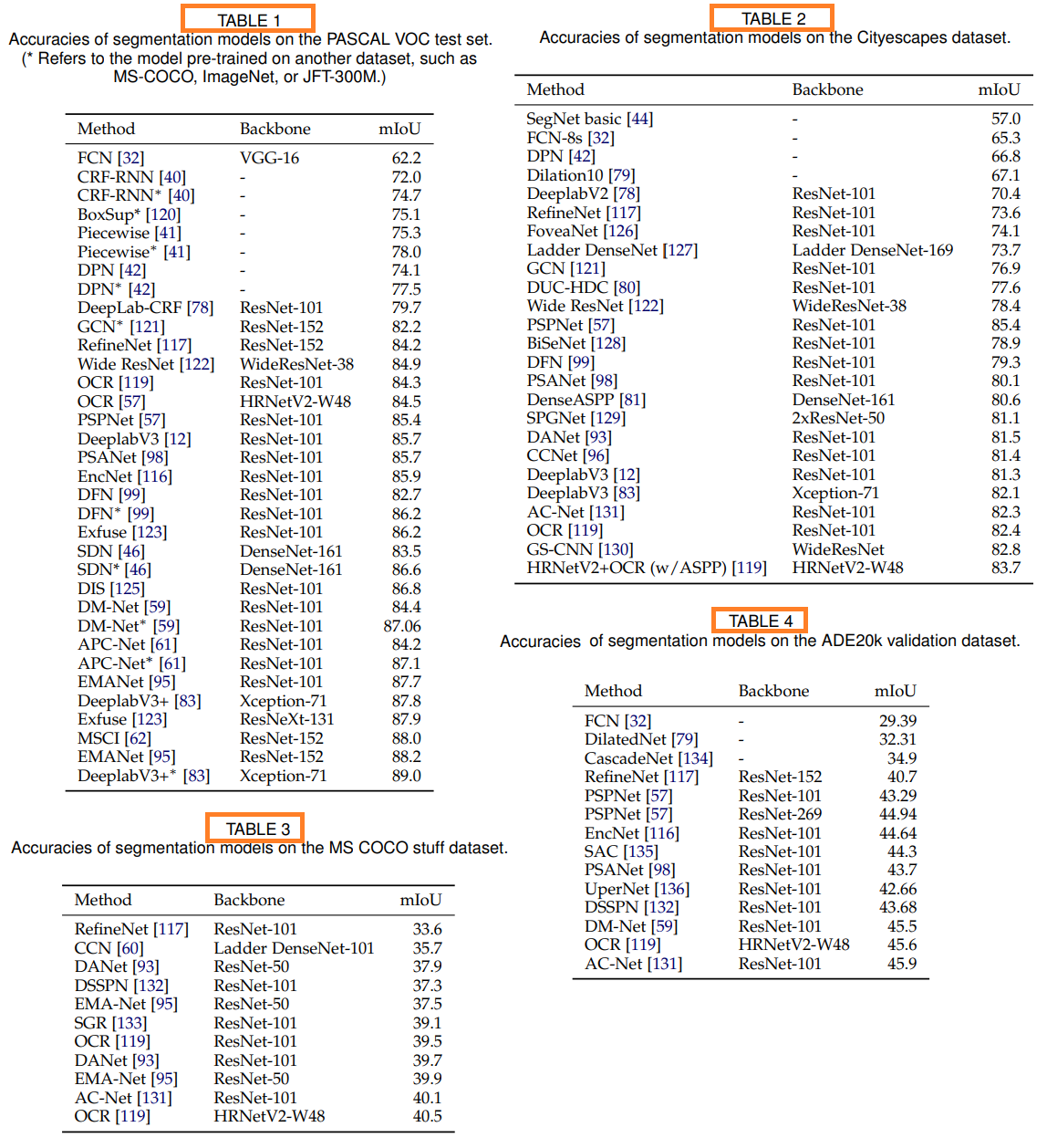
5.2 Quantitative Performance of DL-Based Models
Table1 : the PASCAL VOC
Table2 : the Cityscape test dataset
Table3 : the MS COCO stuff test set
Table4 : the ADE20k validation set
Table5 : the NYUD-v2 and SUNRGBD datasets for RGB-D segmentation (논문 참조)
대부분의 모델에서 코드를 제공하지 않기 때문에, 논문의 내용을 재현하기 위해 많은 노력을 투자했다.
일부 논문에서는 1. performance on non-standard benchmarks, 2. performance only on arbitrary subsets of the test set from a popular benchmark를 발표하고, 적절하고 완벽한 설명을 제공하지 않기 때문에, 실험이 쉽지 않았다.
section 6: CHALLENGES AND OPPORTUNITIES
앞으로 Image segmentation 기술을 향상시키기 위한, 몇가지 유망한 연구방향을 소개한다.
6.1 More Challenging Datasets
large-scale image datasets이 많이 있지만, 더 까다로운 조건과 다양한 종류의 데이터가 필요하다.
객체가 매우 많고나 객체들이 overlapping되어 있는 이미지들이 매우 중요하다.
의료 이미지에서 더 많은 3D이미지 데이터셋이 필요하다.
6.2 Interpretable Deep Models
성능이 좋은 모델들은 많지만, what exactly are deep models learning? / How should we interpret the features learned by these models? 에 대한 답변을 정확히 하지 못하고 있다.
모델들의 구체적인 행동을 충분히 이해하는 연구가 필요하다. 이러한 이해는 더 좋은 모델을 개발하는데 큰 도움을 줄 것이다.
6.3 Weakly-Supervised and Unsupervised Learning
Weakly-supervised (a.k.a. few shot learning)과 unsuper- vised learning은 매우 각광 받고 있는 연구이다. 이 연구를 통해서 Segmentation에서 labeled dataset을 받는데 큰 도움을 받을 수 있을 것이다(특히 의료 분야에서).
The transfer learning(유명한 데이터 셋을 이용해 학습시킨 모델을 이용해 나의 데이터 셋에 맞게 fine-tune하는 것) 과 같이, Self-supervised learning도 우리에게 크게 유용할 것 이다. Self-supervised learning을 통해서 훨씬 적은 수의 데이터셋을 이용해서 Segmentation 모델을 학습시킬 수 있다.
지금은 강화학습을 기반한 Segmentation 모델이 나오고 있지 않지만, 미래에 좋은 기반 방법이 될 수 있을 것이다.
6.4 Real-time Models for Various Applications
최소 25프레임 상의 segmentation 모델을 가지는 것이 중요하다.
이것은 자율주행자동차와 같은 컴퓨터 vision 시스템에 매우 유용할 것이다.
현재 많은 모델들은 frame-rate와 거리가 멀다.
dilated convolution은 the speed of segmentation models을 올리는데 큰 도움을 주지만, 그래도 여전히 개선시켜야할 요지는 많다.
6.5 Memory Efficient Models
많은 모델들은 inference를 하는데도 많은 메모리를 필요로 한다.
휴대폰과 같은 장치에도 적합한 모델을 만들려면 네트워크를 단순화해야한다.
simpler models/ model compression techniques/ knowledge distillation techniques등을 사용해서 더 작은 메모리로 더 효율적으로 복잡한 내트워크를 수정할 수 있다.
6.6 3D Point-Cloud Segmentation
3D 포인트 클라우드 세그멘테이션을 다루는 사람은 훨씬 적다. 하지만 그 관심이 점점 높아지고 있다. 특히 3D modeling, self-driving cars, robotics, building modeling에서.
3D unordered and unstructured data를 처리하기 위해서 CNNs and other classical deep learning architectures를 적용하는것이 가장 좋은 방법인지는 확실하지 않다.
Graph-based deep models이 3D point-cloud segmentation를 다루는데에 좋을 수도 있다.
point-cloud segmentation이 가능하다면 많은 산업적 응용이 가능할 것이다.
# 간단한 2층 Fully connected layer를 구현한.
importnumpyasnp# N is batch size; D_in is input dimension;
# H is hidden dimension; D_out is output dimension.
N,D_in,H,D_out=64,1000,100,10# Create random input and output data
x=np.random.randn(N,D_in)# 64* 1000 -> 64장. 1장당 1000개의 픽셀 데이터 가짐.
y=np.random.randn(N,D_out)# 64* 10
# Randomly initialize weights
w1=np.random.randn(D_in,H)# 1000 * 100
w2=np.random.randn(H,D_out)# 100 * 10
learning_rate=1e-6fortinrange(500):# Forward pass: compute predicted y
h=x.dot(w1)h_relu=np.maximum(h,0)y_pred=h_relu.dot(w2)# Compute and print loss
loss=np.square(y_pred-y).sum()print(t,loss)# Backprop to compute gradients of w1 and w2 with respect to loss
grad_y_pred=2.0*(y_pred-y)grad_w2=h_relu.T.dot(grad_y_pred)grad_h_relu=grad_y_pred.dot(w2.T)grad_h=grad_h_relu.copy()grad_h[h<0]=0grad_w1=x.T.dot(grad_h)# 가중치 갱신 : Update weights
w1-=learning_rate*grad_w1w2-=learning_rate*grad_w2
importtorchdtype=torch.floatdevice=torch.device("cpu")# device = torch.device("cuda:0") # Uncomment this to run on GPU
# N is batch size; D_in is input dimension;
# H is hidden dimension; D_out is output dimension.
N,D_in,H,D_out=64,1000,100,10# Create random input and output data
x=torch.randn(N,D_in,device=device,dtype=dtype)y=torch.randn(N,D_out,device=device,dtype=dtype)# Randomly initialize weights
w1=torch.randn(D_in,H,device=device,dtype=dtype)w2=torch.randn(H,D_out,device=device,dtype=dtype)learning_rate=1e-6fortinrange(500):# Forward pass: compute predicted y
h=x.mm(w1)# https://pytorch.org/docs/stable/torch.html#torch.mm
h_relu=h.clamp(min=0)# https://pytorch.org/docs/stable/tensors.html
y_pred=h_relu.mm(w2)# Compute and print loss
loss=(y_pred-y).pow(2).sum().item()ift%100==99:print(t,loss)# Backprop to compute gradients of w1 and w2 with respect to loss
grad_y_pred=2.0*(y_pred-y)grad_w2=h_relu.t().mm(grad_y_pred)grad_h_relu=grad_y_pred.mm(w2.t())grad_h=grad_h_relu.clone()grad_h[h<0]=0grad_w1=x.t().mm(grad_h)# Update weights using gradient descent
w1-=learning_rate*grad_w1w2-=learning_rate*grad_w2
3. Autograd
위에는 아주 작은 Fully connected layer이므로 backward를 저렇게 손수 구현했지만, 만약 layer가 깊고, 복잡하면 backward를 손수 구현하기 쉽지 않다. Torch에서는 automatic differentiaion 을 제공하므로 자동으로 backward를 사용할 수 있다. Torch에서는 computational graph도 정의해준다.
## 주석을 포함하지 않는 코드 ##
importtorchdtype=torch.floatdevice=torch.device("cpu")N,D_in,H,D_out=64,1000,100,10x=torch.randn(N,D_in,device=device,dtype=dtype)y=torch.randn(N,D_out,device=device,dtype=dtype)w1=torch.randn(D_in,H,device=device,dtype=dtype,requires_grad=True)w2=torch.randn(H,D_out,device=device,dtype=dtype,requires_grad=True)learning_rate=1e-6fortinrange(500):y_pred=x.mm(w1).clamp(min=0).mm(w2)loss=(y_pred-y).pow(2).sum()ift%100==99:print(t,loss.item())loss.backward()withtorch.no_grad():w1-=learning_rate*(w1.grad)w2-=learning_rate*(w2.grad)w1.grad.zero_()w2.grad.zero_()
## 주석을 포함하는 코드 ##
importtorchdtype=torch.floatdevice=torch.device("cpu")# device = torch.device("cuda:0") # Uncomment this to run on GPU
N,D_in,H,D_out=64,1000,100,10# Create random Tensors to hold input and outputs.
# Setting requires_grad=False indicates that we do not need to compute gradients
# with respect to these Tensors during the backward pass.
x=torch.randn(N,D_in,device=device,dtype=dtype)y=torch.randn(N,D_out,device=device,dtype=dtype)# d_loss / d_y를 구할 필요는 없으므로, requires_grad = True로 할 필요 없다.
# Create random Tensors for weights.
# Setting requires_grad=True indicates that we want to compute gradients with
# respect to these Tensors during the backward pass.
w1=torch.randn(D_in,H,device=device,dtype=dtype,requires_grad=True)w2=torch.randn(H,D_out,device=device,dtype=dtype,requires_grad=True)learning_rate=1e-6fortinrange(500):# Forward pass: compute predicted y using operations on Tensors; these
# are exactly the same operations we used to compute the forward pass using
# Tensors, but we do not need to keep references to intermediate values since
# we are not implementing the backward pass by hand.
y_pred=x.mm(w1).clamp(min=0).mm(w2)# Compute and print loss using operations on Tensors.
# Now loss is a Tensor of shape (1,)
# loss.item() gets the scalar value held in the loss.
loss=(y_pred-y).pow(2).sum()ift%100==99:print(t,loss.item())# Use autograd to compute the backward pass. This call will compute the
# gradient of loss with respect to all Tensors with requires_grad=True.
# After this call w1.grad and w2.grad will be Tensors holding the gradient
# of the loss with respect to w1 and w2 respectively.
# requires_grad=True 가 되어 있는 모든 변수(nm)에 대한, 미분 Graph를 따라, d_loss/d_nm를 구해 놓는다.
loss.backward()# Manually update weights using gradient descent. Wrap in torch.no_grad()
# because weights have requires_grad=True, but we don't need to track this in autograd.
# w는 requires_grad가 되어 있기 때문에, 여기서의 연산까지도 grad track할 필요가 없다.
# An alternative way is to operate on weight.data and weight.grad.data.
# 3장의 가중치 갱신 파트를 볼 것.
# Recall that tensor.data gives a tensor that shares the storage with
# tensor, but doesn't track history.
# You can also use torch.optim.SGD to achieve this.
withtorch.no_grad():w1-=learning_rate*w1.gradw2-=learning_rate*w2.grad# Manually zero the gradients after updating weights
w1.grad.zero_()w2.grad.zero_()
4. 새로운 Autograd 기능 정의하기
torch.autograd.Function 를 상속하는 class를 만들어보자. 이러한 class는 새로운 [activation function]을 정의하는데 큰 도움을 준다. 아래에 relu대로 동작하는 class를 직접 만들어 보자.
## 주석을 포함하지 않는 코드 ##
importtorchclassMyReLU(torch.autograd.Function):# staticmethod vs classmethod : http://egloos.zum.com/mcchae/v/11031012
@staticmethoddefforward(ctx,input):ctx.save_for_backward(input)# https://bit.ly/3aHjPoD : torch.autograd.function._ContextMethodMixin.save_for_backward
returninput.clamp(min=0)@staticmethoddefbackward(ctx,grad_output):# relu의 backward는 forward에서 0으로 바꾼것은 backward도 0으로. 나머지는 그대로. 이다.
input,=ctx.saved_tensorsgrad_input=grad_output.clone()grad_input[input<0]=0returngrad_inputdtype=torch.floatdevice=torch.device("cpu")N,D_in,H,D_out=64,1000,100,10x=torch.randn(N,D_in,device=device,dtype=dtype)y=torch.randn(N,D_out,device=device,dtype=dtype)w1=torch.randn(D_in,H,device=device,dtype=dtype,requires_grad=True)w2=torch.randn(H,D_out,device=device,dtype=dtype,requires_grad=True)learning_rate=1e-6fortinrange(500):# https://pytorch.org/docs/stable/autograd.html -> 찾기 : apply
# torch.autograd.Function 를 상속하는 class는 apply함수를 이용해 사용 가능하다
# >> #Use it by calling the apply method:
relu=MyReLU.applyy_pred=relu(x.mm(w1)).mm(w2)loss=(y_pred-y).pow(2).sum()ift%100==99:print(t,loss.item())loss.backward()withtorch.no_grad():w1-=learning_rate*w1.gradw2-=learning_rate*w2.gradw1.grad.zero_()w2.grad.zero_()
## 주석을 포함하는 코드 ##
importtorchclassMyReLU(torch.autograd.Function):"""
We can implement our own custom autograd Functions by subclassing
'torch.autograd.Function' and implementing the forward and backward passes
which operate on Tensors.
"""@staticmethoddefforward(ctx,input):"""
In the forward pass we receive a Tensor containing the input and return
a Tensor containing the output. ctx is 'a context object' that can be used
to stash(저장해두다) information for backward computation. You can cache arbitrary
objects for use in the backward pass using the ctx.save_for_backward method.
"""ctx.save_for_backward(input)# backward를 하기 위해, input을 메모리에 잠시 저장.
returninput.clamp(min=0)@staticmethoddefbackward(ctx,grad_output):"""
In the backward pass we receive a Tensor containing the gradient of the loss
with respect to the output, and we need to compute the gradient of the loss
with respect to the input.
"""input,=ctx.saved_tensorsgrad_input=grad_output.clone()grad_input[input<0]=0returngrad_inputdtype=torch.floatdevice=torch.device("cpu")# device = torch.device("cuda:0") # Uncomment this to run on GPU
N,D_in,H,D_out=64,1000,100,10x=torch.randn(N,D_in,device=device,dtype=dtype)y=torch.randn(N,D_out,device=device,dtype=dtype)w1=torch.randn(D_in,H,device=device,dtype=dtype,requires_grad=True)w2=torch.randn(H,D_out,device=device,dtype=dtype,requires_grad=True)learning_rate=1e-6fortinrange(500):# To apply our Function, we use Function.apply method. We alias this as 'relu'.
relu=MyReLU.apply# Forward pass: compute predicted y using operations; we compute
# ReLU using our custom autograd operation.
y_pred=relu(x.mm(w1)).mm(w2)# Compute and print loss
loss=(y_pred-y).pow(2).sum()ift%100==99:print(t,loss.item())loss.backward()withtorch.no_grad():w1-=learning_rate*w1.gradw2-=learning_rate*w2.gradw1.grad.zero_()이작업을하지않으면,grad가누적된다.w2.grad.zero_()
5. nn 모듈
nn 패키지는 신경망 계층(layer)들과 거의 동일한 Module 의 집합을 정의합니다. 여기서 Module은 입력 Tensor를 받고 출력 Tensor를 계산하는 것은 물론, 학습 가능한 매개변수를 갖는 Tensor 같은 내부 상태(internal state)를 갖습니다.
importtorchN,D_in,H,D_out=64,1000,100,10x=torch.randn(N,D_in)y=torch.randn(N,D_out)# nn 패키지를 사용하여 모델을 순차적 계층(sequence of layers)으로 정의합니다.
# nn.Sequential은 다른 Module들을 포함하는 Module로, 그 Module들을 순차적으로
# 입력으로부터 출력을 계산하고, 내부 Tensor에 가중치와 편향을 저장합니다.
model=torch.nn.Sequential(torch.nn.Linear(D_in,H),torch.nn.ReLU(),torch.nn.Linear(H,D_out),)# 또한 nn 패키지에는 널리 사용하는 손실 함수들에 대한 정의도 포함하고 있습니다;
# 여기에서는 평균 제곱 오차(MSE; Mean Squared Error)를 손실 함수로 사용하겠습니다.
loss_fn=torch.nn.MSELoss(reduction='sum')learning_rate=1e-4fortinrange(500):# 1. forward pass 하기
# 순전파 단계: 모델에 x를 전달하여 예상되는 y 값을 계산합니다. Module 객체는
# __call__ 연산자를 덮어써(override) 함수처럼 호출할 수 있게 합니다.
# 이렇게 함으로써 입력 데이터의 Tensor를 Module에 전달하여 출력 데이터의
# Tensor를 생성합니다.
y_pred=model(x)# 2. Loss값 계산하기
# 손실을 계산하고 출력합니다. 예측한 y와 정답인 y를 갖는 Tensor들을 전달하고,
# 손실 함수는 손실 값을 갖는 Tensor를 반환합니다.
loss=loss_fn(y_pred,y)ift%100==99:print(t,loss.item())# 3. modul 내부의 grad를 0으로 모두 초기화 하고, Backpropagation을 시행한다.
model.zero_grad()# 역전파 단계: 모델의 학습 가능한 모든 매개변수에 대해 손실의 변화도를
# 계산합니다. 내부적으로 각 Module의 매개변수는 requires_grad=True 일 때
# Tensor 내에 저장되므로, 이 호출은 모든 모델의 모든 학습 가능한 매개변수의
# 변화도를 계산하게 됩니다.
# x와 y는 계산할 필요가 없으므로, requires_grad=True로 해주지 않아도 됐다.
# 가중치와 편향은 자동으로 requires_grad=True로 정의된다.
loss.backward()# 4. Backpropagation한 값을 이용해서, 가중치를 갱신한다.
# 경사하강법(gradient descent)를 사용하여 가중치를 갱신합니다. 각 매개변수는
# Tensor이므로 이전에 했던 것과 같이 변화도에 접근할 수 있습니다.
withtorch.no_grad():forparaminmodel.parameters():# 여기서 사용한 메소드. 눈 여겨보기
param-=learning_rate*param.grad
6. Optimizer
지금까지는 모델의 가중치를 직접 갱신했다. {Ex. param -= learning_rate * param.grad} 하지만 우리는 그렇게 할 필요가 없다.
importtorchN,D_in,H,D_out=64,1000,100,10x=torch.randn(N,D_in)y=torch.randn(N,D_out)model=torch.nn.Sequential(torch.nn.Linear(D_in,H),torch.nn.ReLU(),torch.nn.Linear(H,D_out),)loss_fn=torch.nn.MSELoss(reduction='sum')# optim 패키지를 사용하여 모델의 가중치를 갱신할 Optimizer를 정의합니다.
# Adam 생성자의 첫번째 인자는 어떤 Tensor가 갱신되어야 하는지 알려줍니다.
learning_rate=1e-4optimizer=torch.optim.Adam(model.parameters(),lr=learning_rate)fortinrange(500):y_pred=model(x)loss=loss_fn(y_pred,y)ift%100==99:print(t,loss.item())# 역전파 단계 전에, Optimizer 객체를 사용하여 (모델의 학습 가능한 가중치인)
# 갱신할 변수들에 대한 모든 변화도를 0으로 만듭니다. 이렇게 하는 이유는
# 기본적으로 .backward()를 호출할 때마다 변화도가 메모리 버퍼(buffer)에 (덮어쓰지 않고)
# 누적되기 때문입니다. 더 자세한 내용은 torch.autograd.backward에 대한 문서를 참조하세요.
# 따라서 위의 방법이었던, model.zero_grad()를 사용하는게 아닌..
optimizer.zero_grad()# 역전파 단계: 모델의 매개변수에 대한 손실의 변화도를 계산합니다.
loss.backward()# Optimizer의 step 함수를 호출하면 매개변수가 갱신됩니다.
optimizer.step()
7. nn.Module 적극적으로 이용하기
지금까지 model = torch.nn.Sequential를 사용해서 model을 정의했다. 하지만 이렇게 하지 않고 아래와 같은 방법을 사용하는게 복잡한 모델 구성할 때 이롭다.
이 코드를 통채로 외우자!!!!!!!!!!!!!
# 이 코드를 통채로 외우자!!!!!!!!!!!!!
importtorchclassTwoLayerNet(torch.nn.Module):def__init__(self,D_in,H,D_out):super(TwoLayerNet,self).__init__()self.linear1=torch.nn.Linear(D_in,H)self.linear2=torch.nn.Linear(H,D_out)# self.relu1 = torch.nn.ReLU()
defforward(self,x):# self.relu1(self.linear1(x))
h_relu=self.linear1(x).clamp(min=0)y_pred=self.linear2(h_relu)returny_predN,D_in,H,D_out=64,1000,100,10x=torch.randn(N,D_in)y=torch.randn(N,D_out)model=TwoLayerNet(D_in,H,D_out)criterion=torch.nn.MSELoss(reduction='sum')optimizer=torch.optim.SGD(model.parameters(),lr=1e-4)fortinrange(500):y_pred=model(x)loss=criterion(y_pred,y)ift%100==99:print(t,loss.item())optimizer.zero_grad()loss.backward()optimizer.step()
8. 제어 흐름(Control Flow) + 가중치 공유(Weight Sharing)
위와 같이 정직한 Modul을 사용하는게 아닌, 복잡한 모델을 생성해야할 수 있다. 이를 위해서 우리는 아래와 같은 방법을 사용해서 모델을 정의할 수 있다. 여기서는 2번째 Layer의 통과를 0 ~ 3개의 subLayer를 통과하도록 만든다. 가장 안쪽(innermost)의 은닉층들을 계산하기 위해 동일한 가중치를 여러 번 재사용하는 코드를 만들어보자.
importrandomimporttorchclassDynamicNet(torch.nn.Module):def__init__(self,D_in,H,D_out):super(DynamicNet,self).__init__()self.input_linear=torch.nn.Linear(D_in,H)#1 Layer
self.middle_linear=torch.nn.Linear(H,H)#2 Layer : 위 코드와 다르게 이것 추가.
self.output_linear=torch.nn.Linear(H,D_out)#3 Layer
defforward(self,x):"""
모델의 순전파 단계를 정의할 때 반복문이나 조건문과 같은
일반적인 Python 제어 흐름 연산자를 사용할 수 있습니다.
여기에서 연산 그래프를 정의할 때 동일 Module을 여러번 재사용하는 것이
완벽히 안전하다는 것을 알 수 있습니다.
"""h_relu=self.input_linear(x).clamp(min=0)# 1Layer + 1Relu 통과
for_inrange(random.randint(0,3)):# 0 ~ 3 번.2 Layer + 1Relu 를 통과
h_relu=self.middle_linear(h_relu).clamp(min=0)y_pred=self.output_linear(h_relu)# 3Layer를 통과시킨다
returny_predN,D_in,H,D_out=64,1000,100,10x=torch.randn(N,D_in)y=torch.randn(N,D_out)model=DynamicNet(D_in,H,D_out)criterion=torch.nn.MSELoss(reduction='sum')optimizer=torch.optim.SGD(model.parameters(),lr=1e-4,momentum=0.9)fortinrange(500):y_pred=model(x)loss=criterion(y_pred,y)ift%100==99:print(t,loss.item())optimizer.zero_grad()loss.backward()optimizer.step()
여기부터 2019년 이후에 제안된 100가지가 넘는 segmentation methods를 상세히 검토한다.
많은 방법론에서 이것을 사용해서 좋은 성과를 얻었다.
encoder and decoder parts
skip-connections
multi-scale analysis
the use of dilated convolution… more recently
많은 methods를 특징(contributions)로 분류하기는 어렵고, Section2의 방법으로 분류하려한다.
3.1 Fully Convolutional Networks
semantic image segmentation을 위한 최초의 신경망이라고 할 수 있다.
VGG16 및 GoogLeNet를 사용하였고, Fully connected layer와 같이 linear 연산이 아닌 layer를 모두 convolutional layers로 바꾸었다. (fig.7)
임의 사이즈의 input을 받아도 적절한 크기의 segmentation map output을 도출하는 신경망이다.
skip connections을 사용했다. 그러기 위해 upsampling을 적절히 사용하여, [from deep, coarse layers] 정보와 [from shallow, fine layers]정보를 융합하였다. (fig. 8)
PASCAL VOC, NYUDv2, SIFT Flow Dataset에서 SOTA를 달성하였다.
FCN은 지금의 Image Segmentation에서 milestone으로 여겨지지만, 충분히 빠르지 않고, Global context information을 추출하기에 효과적인 모델이 아니다. 그리고 3D이미지로 transferable 하지 않다.(?)
이러한 문제를 해결하기 위해 ParseNet이 등장했다. Global context information에 강하기 위해, he average feature for a layer를 사용하였다. 각 레이어의 특징 맵이 전체 이미지에 풀링되어, context vector가 생성된다. 이것은 정규화하고 언풀링하여 초기 피쳐 맵과 동일한 크기의 새 피쳐 맵을 생성한다. 그런 다음이 특성 맵에 연결된다.(fig9. (c))
FCN은 뇌종양 segmentation [34], instance-aware semantic segmentation [35], 피부 병변 segmentation [36] 및 홍채 segmentation [37]와 같은 다양한 세그먼테이션 문제에 적용되어왔다.
3.2 Convolutional Models With Graphical Models
FCN은 potentially useful scene-level semantic context(잠제적으로 유용한 전체적 정보)를 무시한다. 이러한 문제를 해결하기 위해 CRF (Conditional Random Field) 및 MRF (Markov Random Field)와 같은 확률 적 그래픽 모델을 통합하는 몇가지 방법이 있다.
CNNs and fully connected CRFs을 융합한 chen은 classification을 위해 high level task를 수행하는 depp CNN의 불가변적 속성(?) 때문에 정확한 Segmentation이 이루어지지 않음을 확인하였다. (fig 10)
이러한 deep CNN의 문제를 해결하기 위해, CNN의 마지막 layer결과값과 fully-connected CRF를 결합하였고, 더 높은 정확도(sementation의 경계를 더 정확히 갈랐다.)를 가졌다.
A fully-connected deep structured network for image segmentation. [39],[40]에서는 CNNs and fully-connected CRFs를 end-to-end로 학습시키는 network를 구조화하였다. PASCAL VOC 2012 dataset에서 SOTA 달성했다.
[41]에서 contextual deep CRFs를 이용한 segmentation 알고리즘을 제안했다. 여기서는 contextual 정보를 뽑아내기 위해, “patch-patch”컨텍스트를 (between image regions)와“patch배경”컨텍스트를 사용했다.
[42]에서 high-order relations과 mixture of label contexts를 포함하는, MRFs 정보를 사용하였다. 과거의 MRFs방법과는 달리 deterministic end-to-end learning이 가능한 Parsing Network라는 CNN모델을 제안하였다.
3.3 Encoder-Decoder Based Models
대부분의 DL-based segmentation works에서 encoder-decoder models를 사용했다.
우리는 아래와 같이 2가지 범주로 분류해 모델들을 확인해볼 것이다.
(general segmentation VS Medical and Biomedical segmentation)
3.3.1 Encoder-Decoder Models for General Segmentation
아래의 그림처럼 Deconvolution(= transposed convolution)을 사용한 Segmentation방법의 첫논문이 [43]이와 같다. (fig11) 그림과 같이 encoder와 decoder가 존재하고, decoder에서 deconvolution and unpooling layers를 사용해서 픽셀단위의 레이블링이 이루어진다. PASCAL VOC 2012 dataset에서 (추가 데이터 없이) 좋은 정확도가 도출되었다.
[44] SegNet은 the 13 convolutional layers in the VGG16 network와 구조적으로 동일한 encoder를 사용하였다. (fig12) 가장 중요한 점은 업샘플링을 하며 featrue map을 키울때 encoder에서 max pooling을 했던 그 인덱스를 기억해서 이용하는 것이다. 그리고 SegNet은 다른 모델에 비해서 매개변수가 적다는 장점이 있다.
[45] SegNet의 upgrade version으로 A Bayesian version of SegNet은 encoder-decoder network의 불확실성(upsampling등의 문제)을 해결하고자 노력했다.
최근 개발된 유명한 high-resolution network (HRNet)은 (이전의 고해상도 표현을 복구하려는 DeConvNet, SegNet, U-Net and V-Net과는 조금 다르게) 아래의 사진처럼 고해상, 저해상 이미지와의 정보교환을 이뤄가며 좋은 성능을 얻었다.
최근의 많은 Semantic segmentation 모델들은 contextual models, such as self-attention을 사용하면서, HRNet을 Backbone으로 많이 사용합니다.
지금까지 봤던 Network이 외에도, transposed convolutions, encoder - decoders를 이용하는 최근 모델에는 Stacked Deconvolutional Network (SDN) [46], Linknet [47], W-Net [48], and locality-sensitive deconvolution networks for RGB-D segmentation [49]와 같은 모델들이 있습니다.
3.3.2 Encoder-Decoder Models for Medical and Biomedical Image Segmentation
medical/biomedical image segmentation을 하기 위한 몇가지 모델들을 공부해본다.
FCN과 encoder-decoder를 기본으로 하는 U-Net [50], and V-Net [51]이 의료분야에서 유명하다.
현미경 이미지를 분류하기 위해 U-Net이[50] 개발되었고, 3D medical image(MRI volume) segmentation을 위해서 V-Net[51]이 개발되었다. () (자세한 설명은 논문 참조)
그 외에 Unet은 3D images를 위한 [52], nested Unet[53], road extraction [54]에 많이 사용되었다. 또한 흉부 CT 영상 Progressive Dense V-net (PDV-Net)
3.4 Multi-Scale and Pyramid Network Based Models
주로 Object Detection에서 Multi-scale analysis을 위해서 가장 많이 사용되는 Pyramid Network (FPN) [56]을 중심으로 사용한 모델들을 살펴보자.
FPN은 low and high resolution features를 융합하기 위해서, bottom-up pathway, a top-down pathway and lateral connections방법을 사용합니다. FPN 저자는 Segmentation을 위해서 각 층(다른 해상도 크기의)의 predict단에서 (간단히) 2 layer의 MLP를 사용하였습니다.
[57] PSPN 모델은 (fig17) the global context representation of a scene를 더 잘 이해하기 위해 개발되었다. 특별한 점으로는 ResNet + dilated Network을 사용해서 (b) Featrue Map을 뽑아낸다는 것이다. 그리고 a pyramid pooling module을 사용해서 다른 크기의 pattern(객체)들을 구분해간다. pooling 이후에 1*1 conv를 사용해서 channel을 감소시키고, 마지막 단에는 지금까지의 모든 정보를 concat한 후 conv를 거쳐 픽셀 단위 예측을 수행합니다.
[58]는 고해상도 maps(w,h가 큰)의 skip connection을 이용해서. 저해상도 maps으로 부터 재생성된 segmentation결과에서 경계가 모호한 문제를 해결합니다.
이 외에 Multi-scale analysis를 사용한 모델로 DM-Net (Dynamic Multi-scale Filters Network) [59], Context contrasted network and gated multi-scale aggregation (CCN) [60], Adaptive Pyramid Context Network (APC-Net) [61], Multi-scale context intertwining (MSCI) [62], and salient object segmentation [63]. 등이 있다.
3.5 R-CNN Based Models (for Instance Segmentation)
R-CNN 계열을 이용해 instance segmentation 문제를 해결하는데 많이 사용되었다. 특히 Faster-RCNN은 RPN을 사용해 ROI를 추출한다. 그리고 RoiPool와 CNN을 통해서 객체 위치와 객체 클래스를 유추한다.
Mask R-CNN [65]은 Faster-Rcnn에서 2개의 출력 분기가 아닌, 3개의 출력 분기를 사용하여, 각 객체에 대해서 Instance Segmentation을 수행한다. COCO test set에서 좋은 결과를 도출해 낸다.
Path Aggregation Network (PANet) [66]은 Mask R-CNN과 FPN(The feature extractor)을 기반으로 한다. 위의 사진과 같이 (b), (c)를 사용하는게 특징이고, (e)에서 처럼 Roi를 FCN처리를 하여 the object Mask를 예측한다.
[67]에서는 instances를 구별하고, estimating masks, categorizing objects 하기 위한 multi-task network를 개발한 것이 특징이다. [68]에서는 a novel weight transfer function, a new partially-supervised training paradigm을 사용해서 많은 class instance segmentation수행(label을 정의하지 않은 객체에도, 비지도학습을 이용해서(box의 class값을 사용해서) 새로운 label을 예측하는)을 가능케 한 것이 특징이다.
[69]에서는 Faster-RCNN을 개선한 MaskLab을 개발하였다. Roi에 대해서, semantic and direction prediction를 수행하여, segmentation을 수행하는 것이 특징이다.
[70]에서는 Tensormask를 개발하였다. 이 모델은 dense (sliding window instance) object segmentation에서 좋은 결과를 도출하였다. 4D 상태에서 Prediction을 수행하였고, tensor view를 사용해 Mask-RCNN과 유사한 성능을 가지는 모델을 만들었다.
RCNN을 기반으로 개발된 다른 모델로써, R-FCN [71], DeepMask [72], SharpMask [73], PolarMask [74], and boundary-aware in-stance segmentation [75]와 같은 것들이 있다.
또한 Deep Watershed Transform [76], and Semantic Instance Segmentation via Deep Metric Learning [77]에서 처럼, grouping cues for bottom-up segmentation을 학습함으로써 instance segmentation에서의 문제를 해결하려고 노력했다는 것도 눈여겨 봐야한다.
3.6 Dilated Convolutional Models and DeepLab Family
Dilated convolution(=atrous conv)는 the dilation rate(a spacing between the weights of the kernel w)를 사용한다. 이로써 추가적 비용없이 the receptive field를 키울 수 있었다. 따라서 real-time segmentation에서 많이 사용된다.
Dilated Conv를 사용한 많은 모델들 : the DeepLab family [78], multi-scale context aggregation [79], dense upsampling convolution and hybrid dilatedconvolution (DUC-HDC) [80], densely connected Atrous Spatial Pyramid Pooling (DenseASPP) [81], and the efficient neural network (ENet) [82]
DeepLab2에서는 3가지 주요한 특징이 있다.
max-pooling를 하여 이미지의 해상도(w,h 크기)를 낮추는 대신에 dilated conv를 적극적으로 사용하였다.
Atrous Spatial Pyramid Pooling(ASPP)를 사용해서 multiple scales object를 더 잘 탐사하였다.
객체 경계를 더 잘 구별하기 위해서 deep CNNs and probabilistic graphical models을 사용하였다.
DeepLab은 2012 PASCAL VOC challenge, the PASCAL-Context challenge, the Cityscapes challenge에서 좋은 성능을 내었다. (fig.25)
이후 Deeplabv3[12]에서는 cascaded and parallel modules of dilated convolutions(ASPP{1*1conv를 사용하고 배치 정규화를 사용하는}에서 그룹화된)를 사용하였다.
2018년 이후에 [83]에서 encoder-decoder architecture를 사용한 Deeplabv3+가 새로 발표되었다. 아래 2개의 기술을 사용한 것이 특징이다.
a depthwise convolution (spatial convolution for each channel of the input)로 만들어진, atrous separable convolution
pointwise convolution (1*1 convolution with the depthwise convolution as input)
Deeplabv3+는 DeepLabv3를 encoder 프레임워크(backbone)로 사용하였다. (fig.26)
최근에 수정된 Deeplabv3+ 모델에는 max-pooling와 batch Norm을 사용하지 않고, 더 많은 layers와 dilated depthwise separable convolutions를 사용하는 ‘Xception backbone’를 사용한다.
Deeplabv3+는 the COCO and the JFT datasets을 통해 pretrained 된 모델을 사용하여, the 2012 PASCAL VOC challenge Dataset에서 놓은 성적을 얻었다.
3.7 Recurrent Neural Network Based Models
segmentation을 수행할 때, 픽셀간의 the short/long term dependencies를 모델링할 때 RNN을 사용하는 것도 유용하다. RNN을 사용함으로써 픽셀들이 연결되어 연속적으로 처리된다. 그러므로써 global contexts를 좀 더 잘 찾아내고, semantic segmentation에서의 좋은 성능이 나오게 해준다. RNN을 사용함에 있어 가장 큰 문제점은 이미지가 2D 구조라는 것이다. (RNN은 문자열같은 1차원을 다루는데 특화되어 있으므로.)
[84]에서 Object detection을 위한 ReNet[85]를 기반으로 만들어진 ReSeg라는 모델을 소개한다. 여기서 ReNet은 4개의 RNN으로 구성된다. (상 하 좌 우) 이로써 global information를 유용하게 뽑아낸다. (fig.27)
[86]에서는 (픽셀 레이블의 복잡한 공간 의존성을 고려하여) 2D LSTTM을 사용해서 Segmentaion을 수행했다. 이 모델에서는 classification, segmentation, and context integration 모든 것을 LTTM을 이용한다.(fig.29)
[87]에서는 Graphic LSTM을 이용한 Segmentation모델을 제안한다. 의미적으로 일관된 픽셀 Node를 연결하고, 무 방향(적응적으로 랜덤하게) 그래프를 만든다. (edges로 구분된 그래프가 생성된다.) fig.30을 통해서 Graph LSTM과 basic LSTM을 시각작으로 비교해볼 수 있다. 그리고 Fig31을 통해서 [87]의 전체적 그림을 확인할 수 있다. (자세한 내용은 생략)
DA-RNNs[88]에서는 Depth카메라를 이용해서 3D sementic segmentation을 하는 모델이다. 이 모델에서는 RGB 비디오를 이용한 RNN 신경망을 사용한다. 출력에서는 mapping techniques such as Kinect-Fusion을 사용해서 semantic information into the reconstructed 3D scene를 얻어 낸다.
[89]에서는 CNN&LSTM encode를 사용해서 자연어와 Segmentation과의 융합을 수행했다. 예를 들어 “right woman”이라는 문구와 이미지를 넣으면, 그 문구에 해당하는 영역을 Segmentation해준다. visual and linguistic information를 함께 처리하는 방법을 학습하는 아래와 같은 모델을 구축했다. (fig.33)
LSTM에서는 언어 백터를 encode하는데 사용하고, FCN을 사용해서 이미지의 특성맵을 추출하였다. 그렇게 최종으로는 목표 객체(언어백터에서 말하는)에 대한 Spatial map (fig 34의 가장 오른쪽)을 얻어낸다.
아래의 그림에서, ai : attention vector / ci : context vetor
[90]에서는 multi-scale feature를 사용해서 attention해야할(wdight) 정도를 학습한다. pooling을 적용하는 것보다, attention mechaniism을 사용함으로써 다른 위치 다른 scales(객체크기)에 대한 the importance of features(그 부분을 얼마나 중요하게 집중할지)를 정확하게 판단할 수 있다. (fig. 35)
[91]에서는 일반적인 classifier처럼 labeled된 객체의 의미있는 featrue를 학습하는게 아니라, reverse attention mechanisms(RAN)을 사용한 semantic segmentation방법을 제안하였다. 여기서 RAN은 labeled된 객체만을 학습하는 것이 아닌, 반대의 것들(배경, 객체가 아닌 것)에 대한 개념도 캡처(집중)한다. (fig. 36)
[92]에서는 a Pyramid Attention Network를 사용했다. 따라서 global contextual information을 사용하는데 특화되어 있습니다. 특히 이 모델에서는 dilated convolutions and artificially designed decoder networks를 사용하지 않습니다.
[93]에서는 최근에 개발된 a dual attention network을 사용한 모델을 제안한다. 중심 용어 - rich con-textual dependencies / self-attention mechanism / the semantic inter-dependencies in spatial + channel dimensions / a weighted sum
이 외에도 [94] OCNet(object context pooling), EMANet [95], Criss-Cross Attention Network (CCNet) [96], end-to-end instance segmentation with recurrent attention [97], a point-wise spatial attention network for scene parsing [98], and a discriminative feature network (DFN) [99] 등이 존재한다.
3.9 Generative Models and Adversarial Training
[100]에서는 segmentation을 위해서, adversarial training approach를 제안하였다. (fig. 38)에서 보는 것처럼 Segmentor(지금까지 했던 아무 모델이나 가능) segmentation을 수행하고, Adversarial Network에서 ground-truth와 함께, discriminate를 수행해나간다. 이러한 방법으로 Stanford Background dataset과 PASCAL VOC 2012에서 더 높은 정확성을 갖도록 해준다는 것을 확인했다. (fig. 39)에서 결과 확인 가능하다.
[101]에서는 semi-weakly supervised semantic segmentation using GAN를 제안하였다.
[102]에서는 adversarial network를 사용한 semi-supervised semantic segmentation를 제안하였다. 그들은 FCN discriminator를 사용해서 adversarial network를 구성하였고, 3가지 loss function을 가진다. 1. the segmentation ground truth와 예측한 결과와의 cross-entropy loss 2. discriminator network 3. emi-supervised loss based on the confidence map. (fig. 40)
[103]에서는 의료 영상 분할을 위한 multi-scale L1 Loss를 제안하였다. 그들은 FCN을 사용해서 segmentor를 구성했고, 새로운 adversarial critic network(multi-scale Loss)를 구상했다. critic(discriminator)가 both global and local features에 대한 Loss를 모두 뽑아낸다. (fig.41) 참조.
다른 segmentation models based on adversarial training로는, Cell Image Segmenta-tion Using GANs [104], and segmentation and generation of the invisible parts of objects [105]이 있다.
3.10 CNN Models With Active Contour Models
Active Contour Models (ACMs) [7] 를 기본으로 사용하여, Loss function을 바꾼 새로운 모델들이 새롭게 나오고 있다.
the global energy formulation of [106]
[107] : MRI 영상 분석
[108] : 미세 혈관 이미지 분석
[110] ~ [115]에 대한 간략한 설명은 논문 참조.
3.11 Other Models + Popular Models Timeline
위의 모델을 이외의, DL architectures for segmentation의 몇가지 유명한 모델들을 간략히 소개한다.
[116] ~ [140]
fig. 42는 semantic segmentation를 위한 아주 유명한 모델들을 시간 순으로 설명한다. 지난 몇 년간 개발 된 많은 작품을 고려했을때, 아래의 그림은 가장 대표적인 작품 중에서도 일부만을 보여준다.
# loader하
# transforms 라이브러리는 다음을 참조 : https://pytorch.org/docs/stable/torchvision/transforms.html
transform=transforms.Compose([transforms.ToTensor(),transforms.Normalize((0.5,0.5,0.5),(0.5,0.5,0.5))])# 순서대로 : https://pytorch.org/docs/stable/torchvision/datasets.html#cifar
# : https://pytorch.org/docs/stable/data.html#torch.utils.data.DataLoader <- 위의 글들도 읽으면 좋다.
# torchvision dataset을 이용해서 'Train' dataset가져오기.
trainset=torchvision.datasets.CIFAR10(root='./data',train=True,download=True,transform=transform)trainloader=torch.utils.data.DataLoader(trainset,batch_size=4,shuffle=True,num_workers=2)# torchvision dataset을 이용해서 'Test' dataset가져오기.
testset=torchvision.datasets.CIFAR10(root='./data',train=False,download=True,transform=transform)testloader=torch.utils.data.DataLoader(testset,batch_size=4,shuffle=False,num_workers=2)classes=('plane','car','bird','cat','deer','dog','frog','horse','ship','truck')# trainset, trainloader 로 궁금증 해소해보는것은 나중에 하자..
# 아래의 dataiter를 list화 하고 확인하는 등의 작업을 하면 된다.
Files already downloaded and verified
Files already downloaded and verified
# 심심풀이로, 데이터 한번 확인해보기.
# 1. iter, next 함수 : https://dojang.io/mod/page/view.php?id=2408
importmatplotlib.pyplotaspltimportnumpyasnp# 이미지를 보여주기 위한 함수
defimshow(img):img=img/2+0.5# unnormalize
npimg=img.numpy()plt.imshow(np.transpose(npimg,(1,2,0)))plt.show()# 학습용 이미지를 무작위로 가져오기
# 위에서 사용한 DataLoader를 이런식으로 사용하는 구나.
dataiter=iter(trainloader)images,labels=dataiter.next()# 이미지 보여주기 - 위에서 정의한 imshow 함수를 이용한다.
imshow(torchvision.utils.make_grid(images))# 왜 4장이 오는지 모르겠다.
# 정답(label) 출력
print(' '.join('%5s'%classes[labels[j]]forjinrange(4)))# class 정보의 str을 print 해준다.
dog dog bird horse
2. 합성곱 신경망(Convolution Neural Network) 정의하기
importtorch.nnasnnimporttorch.nn.functionalasFclassNet(nn.Module):def__init__(self):super(Net,self).__init__()self.conv1=nn.Conv2d(3,6,5)# channel 3 -> 6, 5*5 kernel
self.pool=nn.MaxPool2d(2,2)# kennel 2 , stride 2
self.conv2=nn.Conv2d(6,16,5)# 이후 최종 output size = 16c * 5h * 5w
self.fc1=nn.Linear(16*5*5,120)self.fc2=nn.Linear(120,84)self.fc3=nn.Linear(84,10)defforward(self,x):# print('input x 의 사이즈는 (배치까지 고려하여...) :' ,x.size())
x=self.pool(F.relu(self.conv1(x)))x=self.pool(F.relu(self.conv2(x)))x=x.view(-1,16*5*5)x=F.relu(self.fc1(x))x=F.relu(self.fc2(x))x=self.fc3(x)returnxnet=Net()# print(net)
3. 손실 함수와 Optimizer 정의하기
importtorch.optimasoptimcriterion=nn.CrossEntropyLoss()# 나중에 이런 식으로 loss를 정의할 예정이다. loss = criterion(out, target)
optimizer=optim.SGD(net.parameters(),lr=0.001,momentum=0.9)# 그리고 나중에 loss.backward(); optimizer.step(); 를 할 예정
4. 신경망 학습하기
total=0forepochinrange(2):# loop over the dataset multiple times
running_loss=0.0fori,datainenumerate(trainloader,0):# enumerate(iter variable,))for문을 돌기 시작할 index를 적는다.
# get the inputs; data is a list of [inputs, labels]
inputs,labels=datatotal+=labels.size(0)# zero the parameter gradients
optimizer.zero_grad()# forward + backward + optimize
outputs=net(inputs)loss=criterion(outputs,labels)loss.backward()optimizer.step()# print statistics
running_loss+=loss.item()# 2000 mini-batches의 모든 loss를 합친다.
ifi%2000==1999:# print every 2000 mini-batches
# print('input size, type : {}, {} , labels : {}'.format(inputs.size(), type(inputs), labels))
print('[%d, %5d] loss: %.3f'%(epoch+1,i+1,running_loss/2000))running_loss=0.0print('total image : %d장'%(total))# -> 50000장
print('Finished Training! total image : %d 장'%(total))
input size, type : torch.Size([4, 3, 32, 32]), <class ‘torch.Tensor’> , labels : tensor([2, 2, 2, 1]) 이것으로 보아, 4장의 이미지를 미니 배치로 사용한다. labels는 4장의 이미지 각각의 class를 0~9를 사용해 표현했다. [1, 2000] loss: 2.190 [1, 4000] loss: 1.826 [1, 8000] loss: 1.568 [1, 12000] loss: 1.427 print(‘total image : %d장’%(total)) [2, 4000] loss: 1.353
Finished Training! total image : 100000 장
추가 중요 팁! : jupyter notebook 에서 위의 cell을 계속 다시 실행하면, 학습이 누적된다.
# 학습시킨 모델 가중치 모두 저장하기 https://pytorch.org/docs/stable/nn.html?highlight=state_dict#torch.nn.Module.state_dict
PATH='./cifar_net.pth'# pytorch에서는 가중치를 저장하는 파일로, pth를 사용하는 구나.
torch.save(net.state_dict(),PATH)
5. Test용 데이터로 신경망 검사하기
# testloader를 이용해서 test이미지를 가져와서 사진과, 정답 labels을 확인해보자
dataiter=iter(testloader)# 이렇게 iter를 사용할 필요가 없다. 1개의 mini-batch에 대한 평가만 하려고 하는 짓거리다.
images,labels=dataiter.next()# images, labels = dataiter.next().next()
# print images
imshow(torchvision.utils.make_grid(images))# print labels
print('GroundTruth: ',' '.join('%5s'%classes[labels[j]]forjinrange(4)))
# 전체 데이터 셋에 대해서 accuracy를 판단해보자.
correct=0total=0withtorch.no_grad():# 2장에서 배웠던, 이것을 Evaluation 하거나, Test 데이터 확인할 때 사용하는구나!
fordataintestloader:# 위에서 처럼 iter를 사용하지 않고 이렇게 편하게 사용하면 된다.
# 1개의 mini-batch를 평가할 때와 똑같은 방법으로 (바로 위의 방법) 똑같이 하면 된다.)
images,labels=dataoutputs=net(images)_,predicted=torch.max(outputs.data,1)total+=labels.size(0)# 몇장의 사진을 예측했는지. 즉 labels.size(0) == 4 이므로 4를 계속 더해간다.
correct+=(predicted==labels).sum().item()# 4개 중 몇개를 맞췄는지 확인한다.
# 내가 가진 testloader의 data가 없어질 때까지 과정을 반복한다.
print('Accuracy of the network on the 10000 test images: %5d %% / total : %5d '%(100*correct/total,total))
Accuracy of the network on the 10000 test images: 54 % / total : 10000
# 각 class/label 별로, accuracy가 어떻게 되는지, 분류해서 확인해보자
# 신경망 통과는 당연히 다시해댜한다 ^^
class_correct=list(0.foriinrange(10))class_total=list(0.foriinrange(10))withtorch.no_grad():fordataintestloader:images,labels=dataoutputs=net(images)_,predicted=torch.max(outputs,1)c=(predicted==labels).squeeze()foriinrange(4):label=labels[i]class_correct[label]+=c[i].item()class_total[label]+=1foriinrange(10):print('Accuracy of %5s : %2d %%'%(classes[i],100*class_correct[i]/class_total[i]))
Accuracy of plane : 67 %
Accuracy of   car : 76 %
Accuracy of  bird : 53 %
Accuracy of   cat : 50 %
Accuracy of  deer : 39 %
Accuracy of   dog : 29 %
Accuracy of  frog : 51 %
Accuracy of horse : 57 %
Accuracy of  ship : 68 %
Accuracy of truck : 57 %
  File "<ipython-input-13-b15bb06280db>", line 1
    Tensor를 GPU로 이동했던 것처럼, 신경망 또한 GPU로 옮길 수 있습니다.(1장에서 배움)
               ^
SyntaxError: invalid syntax
device=torch.device("cuda:0"iftorch.cuda.is_available()else"cpu")# CUDA 기기가 존재한다면, 아래 코드가 CUDA 장치를 출력합니다:
print(device)# >> cuda:0
# 아래를 통해 재귀적으로 모든 모듈의 매개변수와 버퍼를 CUDA tensor로 변경합니다!!
net.to(device)
# 주의할점!! 각 단계에서 입력(input)과 정답(target)도 GPU로 보내야 한다는 것도 기억해야 합니다:
## 위에서 이렇게 활용하는 부분에서.. for i, data in enumerate(trainloader, 0):
inputs,labels=data[0].to(device),data[1].to(device)


 -
-