【GPU_Server】 Google Cloud 플랫폼 - 적절한 conda 환경 Tensorflow, Keras 버전 맞추기

딥러닝을 위한 적절한 아나콘다 환경 셋팅하기

이전 게시물을 보고 오시는 것을 추천드립니다.

1. Tensorflow & Keras 버전 세팅 방법

  • 참고자료
    image
  • 추천하는 3가지 가상환경 :
    1. tf113 : Tensorflow 1.13, Keras 2.2
    2. tf115 : Tensorflow 1.15, Keras 2.3
    3. tf_obj : Tensorflow 1.15, Keras 2.3 -> Tensorflow object dection API 사용하기 위한 Env
  • 아래의 코드 참고할 것

      $ conda create -n tf113 python=3.6
      $ conda activate tf113
      $ cd envs/tf113/lib/python3.6   -> python3.6 설치
      $ cd ./site-packages  -> 기본 package들이 설치되어 있다. 
      $ cd ~/DLCV/data/util/
      $ chmod +x *.sh
      $ ./install_tf113.sh  (중간에 에러나오는거 무시 - 버전 맞춰주는 것)
    
      $ ps -ef | grep jupyter 
      - jupyter lab 말고 /계정ID/anaconda3 jupyter PID 
      $ kill -9 PID
      $ conda activate tf113
      $ cd ~/ && ./start_jn.sh         
      - jupyter의 목록에 conda 라는 목록이 추가된 것을 확인할 수 있다. 
    
  • 새로운 conda env를 사용해서 jupyter를 열고 싶으면 다음을 꼭 설치해야 한다.

      # DLCV/blob/master/data/util/install_tf113.sh 참조
      $ conda install -c conda-forge pycocotools -y
      $ conda install nb_conda -y
    
      # for  multi jupyter notebook kernal
      $ pip install ipykernel
      $ python -m ipykernel install --user --name <Conda Eev Name>
    
  • install_tf113.sh 내부에 있는 코드 중 $ conda install nb_conda -y 명령어를 통해서 콘다 환경들에게 별도로 jupyter를 따로 실행할 수 있게 해준다.
  • 여러개의 conda 가상환경에서 Jupyter를 열 때. kernel을 골라달라고 창이 뜰 수도 있다. 이때 tf113을 잘 골라주면 된다. 자주 나오니까 각 버전에 맞는 kernel 환경을 선택해 주면 된다. 선택할 kernel 이름이 있는 이유는 install.sh부분에 ‘$ python -m ipykernel install –user –name tf113’이 있기 때문에 이름이 있는거다. env여서 이름이 뜨는게 아니라 커널 설정을 해줬기 때문에 이름이 뜨는 거다. (Jypyter에서 Python [conda env:tf113] 와 같은 노투븍 커널 셋팅을 할 수 있도록!)

image

  • retinaNet에서 tf115를 사용하니까, 그때는 원래 띄어진 Jypyter를 죽이고 activate tf115 를 한 후 start_jn.sh를 실행한다.

2. 구글 클라우드 $300 무료 크레딧 효과적 사용법

  1. 결재 - 개요에 자주 들어가기
  2. 결제 - 예산 및 알림 - 알림 설정하기
  3. 결제 - 거래 - 자주 들어가서 확인하기
    • 300 GB storage PD capacity 한달에 14,000원 계속 나간다.
    • CPU core, Static ip(고정 ip) charging 등 돈이 추가적으로 많이 들어간다.
  4. GPU 서버를 항상 내리는 습관을 가지도록 하자. (VM instance 중지 및 정지)
  5. GPU 사용량, Setup 하는 자세를 배우는 것도 매우 필요하다.
  6. 구글 클라우드 서비스 모두 삭제하는 방법
    • instance 중지 - 삭제 - 서버 및 storage 비용은 안나간다
    • VPC network - 외부 IP 주소 - 고정 주소 해제 (이것도 매달 8천원 나간다.. )
    • Strage - 브라우저 - object storage 삭제
    • 프로젝트 설정 - 종료 (모든 결제 및 트래픽 전달 중지 된다) 7 결제 자주 확인하기
      image

3. Cloud 사용시 주의사항 및 Object Storage 설정

  1. 오류 해결 방법
    • GPU resources 부족 = 기다려라. 하루정도 기다리면 문제 해결 가능
    • 심각한 문제가 발생하면 VM instance 지우고 다시 설치 및 Setup하는 자세 및 습관을 들여라.
  2. Object Storage 설정하기
    • 작업을 편하기 하기 위해서 설정해두면 편리하다.
    • storage - 브라우저 - 버킷 생성 - 단일 region 및 설정 - default 설정 - 저장
    • 접근 인증을 받아야 한다. - server에서 object storage 에 붙기위해서 몇가지 설정이 필요.

        gsutil : google cloud와 연동되어 쉽게 이용할 수 있는 터미널 명령어
        $ gsutil ls gs://my_budcker_Name
        - 아직 권한이 없는 것을 확인할 수 있다. 
      
    • object storage 세부정보 - 권한 - 구성원추가 - 계정이메일 추가, 역할 Storage 저장소 관리자, 저장 - 이제 storage 에 등록을 했다. 하지만 server 인증을 받아야 한다.

        $ gcloud auth login
        - Yes
        - link copy
        - 웹 도메인에 paste - 로그인 및 코드 복사
        - SSH에서 Enter verification code
        $ gsutil ls gs://my_budcker_Name    -> 이제 여기 접근 가능
        $ qsutil cp <file Name> gs://my_budcker_Name    -> 이런식으로 bucket(object storage)에 접근 가능
      
    • winSCP를 사용해서 Putty와 연동 및 파일 업로드 가능
      • winSCP 다운로드 및 설치
      • 로그인 - 도구 - 가져오기 - Putty 원하는 환경 선택
      • 파일 업로드가 매우 쉽게 가능
      • image

4. Colab을 이용한 실습 환경 구축하기

  1. 런타임 유형 - GPU 설정 주의
  2. tensorflow 1.13에서 동작이 안되므로, tensorflow 1.15 설치하기.
  3. % cd, ! terminal command 와 같이 %와 !를 적절히 사용해라.
  4. google drive mount 해서 사용하기
    image

【GPU_Server】 Google Cloud 플랫폼 - VM instance Jupyter로 이용하기

무료로 150시간 정도 편리하게 GPU를 사용할 수 있는 Google Cloud 딥러닝 플렛폼 활용 방법

Google Cloud 딥러닝 플렛폼 이용하기

Google Cloud VS Colab

  • Colab을 사용해도 좋지만, Google Cloud를 사용하는 것이 빠르고 편리하므로 이것을 사용하는 방법에 대해서 공부할 계획이다.
  • 다양한 데이터를 사용해서, 다양한 모델을 사용해서 공부해볼 예정이다.

1. Google cloud platform 가입하고 활용하기

  • google cloud platform 사이트 바로가기
  • 콘솔 -> 서비스 약관 확인하기
  • 무료로 가입하기 -> 서비스 약관 확인하기
  • 무료계정이면 GPU를 사용할 수 없다. 자동 결제를 등록해서 유료계정으로 만들어야 GPU사용가능
  • Computer Engine -> VM 인스턴드 생성하기. 설정은 아래와 같이.
    image
  • 유료 계정으로 업데이트 -> GPU 할당 메일 보니게 -> GPU할당하기
  • 다시 VM 인스턴트 생성하기 - T4(추천), P100과 같은 GPU할당하는 인스턴트로 생성하기(운영체제 : 딥러닝 리눅스) -> 인스탄스 생성 안됨 -> 메일 보내야 함. -> IAM 및 관리자 - 할당량 - GPUs all region - 할당량 수정 - 메일 보내기 - 확인 답변 받고 인스턴트 재생성 (최근 메일에 대한 GPU 할당 거절이 많다. CPU서버를 48시간 이상 가동 후 요청을 다시 해보는 것을 추천한다.)
    image
  • 우선 Colab에서 작업하고 있자. Colab에서 나의 google drive와 마운트하고 그리고 작업을 수행하자. 코랩 오래 할당시 주의할 점 (런타임 연결 끊김 방지 정보)

2. Google cloud platform 이란. + Port Open하기.

  • 다음의 동영상(Youtube링크)을 보고 공부한 내용을 기록합니다,
    1. 구글 클라우드플랫폼 입문 활용
    • 아마존 AWS와 MS Azure 서비스와 비슷한 서비스이다. 하지만 경쟁사 서비스보다 늦게 시작했기 때문에 가성비가 좋다. 그리고 용어 하나하나가 AWS보다 이해가 쉽다는 장점이 있다.
    • 프로젝트 단위로 움직이다. 프로젝트당 Computers, VM 인스턴스들, Docker들을 묶음으로 사용할 수 있다. 프로젝트를 크게 한다고 하면 한달에 40만원이면 아주 편하게 사용할 수 있기 때문에 매우 유용하다.
    • 컴퓨팅 - 컴퓨터 엔진, 쿠버네틱스 엔진, 클라우드 Function, 클라우드 Run 등 가장 중요한 요소들이 존재한다.
    • 이 중 컴퓨터 엔진의 VM instance를 가장 많이 사용하게 되고 이 인스턴트 하나가 가상 컴퓨터 하나(하나의 기본적은 자원)라고 생각하면 편하다.
    • VM instance : Region(GPU, CPU 하드웨어가 있는 지역), 영역, 시리즈, 용도들을 선택하면서 가격이 변화하는 것을 확인할 수 있다. GPU를 사용하면 비용이 많이 든다. Colab에서는 무료로 GPU를 사용할 수 있기 때문에 Colab을 사용하는 것이 유용하다.
    • VM instance 설정 : 엑세스 범위를 설정해서 인스턴트 끼리의 연결, 공유를 가능하며 방화벽 설정은 무조건적으로 체크하는 것이 좋다. (나중에 바꿀 수 있다) 보안, 가용성 정책을 사용하면 가격이 저렴해지나 리소스가 전체적으로 부족해지면 리소스가 뺏길 수도 있다.
    • VM instance 생성 완료 : 외부 IP는 가변적이다. 알아두자. 내부 IP는 같은 Region의 인스턴트끼리 소통할 수 있는 IP이다.
  1. 인스턴트 SSH 접속과 도커 서비스, 방화벽 규칙
    • SSH에 접근하는 방법은 SSH를 클릭하거나, 다른 외부 SSH에서 접속하기, 웹으로 접속하기 3가지 방법이 있다. 아래의 방법을 통해서 웹으로 접속 설정을 해보자.
    • SSH 접속을 통해서 우분투와 접근할 수 있다. SSH-브라우저창 열기를 하면 Terminal을 쉽게 열 수 있다. apache2를 설치할 것(80/TCP로 웹서비스 사용 가능). git을 설치할 것.

    • $ sudo apt update
      $ sudo apt-get install apache2
      $ sudo service apache2 start
      $ sudo apt-get install git
      $ sudo netstat -na | grep 80
      
    • 외부 IP 클릭! -> 주소창 http 지우기 -> Apache2 Debian Default Page 확인 가능. Apache2를 그대로 사용하지 않고 Docker환경을 이용해서 어플리케이션 올릴 예정
    • Docker설치가 안되면 https://docs.docker.com/engine/install/debian/ 여기서! 우분투 아니라 데비안이다! 그리고 apt-get update에서 docker fetch 문제가 있어도 “ sudo apt-get install docker-ce docker-ce-cli containerd.io “ 걍 해도 잘 동작하는 것 확인 가능.

        $ sudo apt install docker.io
      
        $ sudo docker search bwapp
        $ sudo docker pull raesene/bwapp (또는 wordpress)
        $ sudo docker run -d --name webconnet -p 81:80 raesene/bwap
      
    • 이제 웹에서 외부 IP:81 로 들어가준다. 하지만 들어가지지 않은 것을 확인할 수 있다. 이것은 구글 클라우드에서 방화벽 처리를 해놓았기 때문이다.
    • Google Cloud Platform - VPC 네트워크 - 방화벽 - 방화벽 규칙 만들기 - 소스 IP 범위 : 0.0.0.0/0 tcp: 81 정의 - 그리고 다시 외부 IP:81로 접근하면 아래와 같은 화면 결과.
      image
    • 외부 IP:81/install.php 로 들어가면 bwapp(웹해킹)사이트로 들어갈 수 있다.

    • 나는 이 방법을 사용해서 8080 port의 방화벽을 허용해 놓고, ml-workspace Image를 가져와서 Container를 실행했다. 다음과 같은 명령어를 사용했다.

      $ sudo docker run -d \
      -p 8080:8080 \
      --name "ml-workspace" -v "${PWD}:/workspace" \
      --env AUTHENTICATE_VIA_JUPYTER="eoqkr" \
      --restart always \
      mltooling/ml-workspace:latest
      
    1. GCP의 MarektPlace 활용하기. 저장 디시크 활용

3. 딥러닝용 가상환경 구축하기

  • 1에서 GPU 할당을 받았다 그 후 작업하는 과정을 요약해 놓는다.
  • 아래의 과정은 SSH 크롬 브라우저를 사용해도 되지만, 고정 IP를 사용해서 Putty로 쉽게 윈도우에서 연결할 수 있도록 설정하는 방법을 적어 놓은 것이다. (Google cloud vm instance Putty connect 등으로 구글링하면 나올 내용들을 정리해 놓는다.)
    1. 4코어 15GB 메모리. GPU T4 1개. 부팅디스크 (Deep Learning on Linux) 디스크 300GB.
    2. Cloud 서버 활용하기 - IP설정(고정적으로 만들기) : VPC 네트워크 - 외부 IP주소 - 고정 주소 예약 (region-연결대상 만 맞춰주고 나머지는 Default로 저장)
    3. 방화벽 규칙 - 방화벽 규칙 만들기 - 8888 port 열기 - 네트워크의 모든 인스턴스 - tcp:8888 ->
    4. Putty donwnload - Putty gen (Private Key 만드는데 사용) 열기 - 인스턴스 세부정보 수정 - Key generate(Key comment : 구글 계정 아이디 넣기) - Key 복사해서 SSH 키 입력 - (Putty gen) Save private, public key - VM 인스턴스 세부정보 수정 저장.
    5. 외부 IP를 Putty에 넣어주고, SSH Auth Browsd - 위에 저장한 Private key 클릭 - Host Name을 sb020518@외부IP 로 저장하고 save_sessions - Open.
    6. Nvidia driver 설치 Yes. - Nvidia driver installed - nvidia-smi 체크해보기
    7. Nvidia driver가 잘 설치되지 않는다면 다음의 과정을 거친다.
      $ cd /opt/deeplearning
      $ sudo ./install-driver.sh
    

4. 주피터 노트북 Setup 하기

  • 실습을 위한 코드를 다운 받고, 아나콘다를 설치 후. Jupyter server를 설치한다.
  • 아래의 과정을 순서대로 수행하면 된다.

      $ git clone ~~culminkw/DLCV
      - anaconda download 하기.(wget 링크주소복사 및 붙여넣기)
      $ chmod 777 ./Anaconda3
      - 콘다 설치 완료
      $ cd ~/
      $ jupyter notebook --generate-config
      $ cd ~/.jupyter
      $ vi ~/.vimrc   ->   syntax off  -> :wq!  (편집창 색깔 이쁘게)
      $ vi ~/.jupyter/.jupyter*.py   ->   DLCV/data/util/jupyer_notebook_config.py 의 내용 복붙 해놓기 
      - (차이점을 비교해서 뭐가 다른지 공부하는 시간가지기 Ex.외부포트 공개, 비밀번호 없음 등... )
      $ cd && vi start_jn.sh    ->  nohup jupyter notebook &  (back End에서 실행)
      $ chmod +x start_jn.sh
      $ ./start_jn.sh
      $ tail -f nohup.out   (jupyter 실행라인이 보여야 함)
      - http:// VM instance 외부-IP:8888  (https 아님)
      - jupyter 실행되는 것을 볼 수 있다. 
    

    image

  • 이와 같이 우리의 SSH 환경이 jupyter에서 실행되는 것을 확인할 수 있다.

5. GCP tensorboard 열기

  • GCP의 SSH를 이용하는 경우
    1. SSH를 GCP를 통해서 열어서 $ tensorboard –logdir=runs 실행
    2. TensorBoard 2.2.1 at http://localhost:6006/ (Press CTRL+C to quit)
      라고 나오면 이떄 나오는 링크를 클릭해서 들어가야 tensorboard를 볼 수 있다.
    3. 참고했던 사이트 이 작업을 해서 되는건지 아닌지는 모르겠다. 이거 했을 때 에러가 많았는데…
    4. 인스턴스_외부_IP:6006/ 와 같은 링크로 크롬에 직접 쳐서는 들어갈 수 없다.
  • jupyter notebook의 terminal를 이용하는 경우
    1. 이상하게 jupyter notebook을 틀어서 위와 같은 작업을 똑같이 실행하면
      • localhost:6006/로 들어갈 수 없다
      • 실행하던 terminal이 멈처버린다. ctrl+c도 안 먹힌다.
      • terminal을 shortdown할 수도 없다.
    2. 내 생각인데, 인스턴스_외부_IP:8888에서 다시 6006을 열라고 하니까 안되는 것 같다.
      • 주인이 있는데, 고객이 고객을 상대하려고 하는 꼴인건가??
    3. 옛날에 은환이가 하던 jupyter 메뉴에서 tensorboard를 여는 방법은, 은환이 왈, ‘jupyter notebook에서 tensorboard와 연동이 안되어 있을 거다.’ 나중에 jupyter에서 tensorboard를 여는 방법은 연동을 해서 할 수 있도록 찾아보자. (ml_workspace 에서 할 수 있는 것처럼.)
    4. jupyter로 작업하는 동안, vscode와 GCP로 tensorboard를 열려고 하면 event파일을 다른 프로세서에서 잡고 있기 때문에 열 수 없다. 따라서, 주피터 cell에다가 ! tensorboard –logdir=runs 를 치고 localhost로 들어가면 된다. 신기하게 여기서 localhost도 내 노트북 IP를 사용한다.
    5. 근데 4번처럼 하면 다른 셀을 실행할 수가 없다. 개같다…
  • vscode를 이용하는 경우
    1. terminal에서 $ tensorboard –logdir=runs 실행하면, localhost:6006링크를 준다.
    2. 그리고 그 링크를 클릭하면, 나의 노트북 ip를 이용해서(신기방기) tensorboard를 열어준다!!
    3. 이게 GCP SSH 보다 훨씬 편할 듯 하다!
  • 최종방법!
    1. 다음 사이트를 참고 했다. jupyter에서 tensorboard 사용법
    2. ‘vision’ conda env에서 pip install jupyter-tensorboard 실행(conda install 없다.)
    3. 성공!
      image

6. GPU 할당 받은 instance 만들기

  1. GPU 할당은 받았다. 하지만 Credit을 사용하고 있어서 GPU instance 만들기 불가능
  2. $ gcloud computer 를 사용하는, google console 을 사용해보기로 했다.
  3. 다음과 같은 명령어를 사용했다. 걸리는 점은 image project와 family설정을 아무리 해줘도, cuda가 이미 잘 설치된 image는 설정이 불가능하더라. GCP image document
    gcloud compute instances create p100-1 \
    --machine-type e2-standard-2 --zone us-west1-b \
    --accelerator type=nvidia-tesla-p100,count=1 \
    --image-family debian-9  --image-project debian-cloud   \
     --restart-on-failure 
    # [--preemptible] 다른 사람이 사용하면 나의 GPU를 뺏기게 가능하게 설정 But 저렴한 가격으로 GPU 사용가능

    >> ERROR: (gcloud.compute.instances.create) Could not fetch resource:
    >> - Instances with guest accelerators do not support live migration.
  1. 결국 나는 guest 이므로 accelerators (GPU) 사용 불가능. 하…

7. snapshot 과 image를 이용해서 vm-instance 복사 및 저장하기

  1. snapshot 만들기
  2. Image 만들기
  3. 프로젝트 구성원 추가하기
  4. 다른 계정에서 인스턴스 만들기
  5. 이미지 선택 -> 맞춤 이미지 -> 프로젝트 선택 -> 아까 만든 이미지 선택
  6. 이미지 공유 성공!(공유는 불가능하고 migration은 가능하다)

【Ubuntu】 노마드 코더의 윈도우 10 개발환경 구축

참고 사이트 : 노마드 코더의 윈도우 10 개발환경 구축
이 과정을 메모리가 좀 더 높은 컴퓨터에 하고 싶은데… 지금 새로운 것을 사서 하기도 그렇고 일단 삼성 노트북 팬s에서 잘해보고 나중에 컴퓨터 새로 사면 또 다시 설치 잘 해보자^^

## [Final setting Image] img

1. Setup

  1. windows Update
    windows 10 - 2004 버전까지 업데이트가 되어있어야 WSL를 사용가능하다.
  2. VScode
    vscode를 설치하고 다양한 extension을 설치하면 좋다.
    예를 들어서 나는 material Theme, material theme icons, prettier등이 좋았다.
  3. Chocolatey
    우리가 우분투에서 프로그램을 설치하려면
    $ sudo apt-get install kolourpaint4
    를 하면 쉽게 설치할 수 있었다. 윈도우에서도 이렇게 할수 있게 해주는게 Chocolatey이다. 설치방법은 간단하고, 이제 windows powershell에서 Find packages에서 알려주는 명령어를 그냥 복사, 붙여넣기하면 프로그램 설치를 매우 쉽게 할 수 있다. 그럼에도 불구하고 이것보다 Linux환경을 사용하는 것을 더욱 추천한다.
  4. windows terminal
    MS store에서 다운받을 수 있는 터미널. 그리거 여기 WSL를 파워셀에 써넣어서 리눅스 계열 OS(Ubunutu) 설치할 수 있게 해준다. 그리고 MS store에 들어가서 Ubuntu를 설치해준다.(다시시작 반복 할 것)
    설치 후 바로 위의 사이트의 ‘~옵션 구성 요소 사용’, ‘~기본 버전 설정’, ‘~WSL 2로 설정’등을 그대로 수행한다.

2. Terminal Customization

  1. $ sudo apt install zsh
  2. 사이트의 bash install을 이용해 우분투에 설치. curl, wget 이용한 설치든 상관없음.
  3. Oh my zsh 설치완료.
  4. 터미널 테마 변경하기
    이 사이트를 이용해서 새로운 schems를 만들어주고 colorScheme을 변경해주면 좋다.
            
     // To view the default settings, hold "alt" while clicking on the "Settings" button.
     // For documentation on these settings, see: https://aka.ms/terminal-documentation
    
     {
         "$schema": "https://aka.ms/terminal-profiles-schema",
    
         "defaultProfile": "{c6eaf9f4-32a7-5fdc-b5cf-066e8a4b1e40}",
    
         "profiles":
         {
             "defaults":
             {
                     "fontFace" : "MesloLGS NF"
             },
             "list":
             [
                
                 {
                     // Make changes here to the powershell.exe profile
                     "guid": "{61c54bbd-c2c6-5271-96e7-009a87ff44bf}",
                     "name": "Windows PowerShell",
                     "commandline": "powershell.exe",
                     "hidden": false,
                     "colorScheme" : "Monokai Night"
                 },
                 {
                     // Make changes here to the cmd.exe profile
                     "guid": "{0caa0dad-35be-5f56-a8ff-afceeeaa6101}",
                     "name": "cmd",
                     "commandline": "cmd.exe",
                     "hidden": true
                 },
                 {
                     "guid": "{b453ae62-4e3d-5e58-b989-0a998ec441b8}",
                     "hidden": true,
                     "name": "Azure Cloud Shell",
                     "source": "Windows.Terminal.Azure"
                 },
                 {
                     "guid": "{c6eaf9f4-32a7-5fdc-b5cf-066e8a4b1e40}",
                     "hidden": false,
                     "name": "Ubuntu-18.04",
                     "source": "Windows.Terminal.Wsl",
                     "colorScheme" : "VSCode Theme for Windows Terminal"
                 }


             ]
         },
    
         // Add custom color schemes to this array
         "schemes": [
             {
                 "name" : "Monokai Night",
                 "background" : "#1f1f1f",
                 "foreground" : "#f8f8f8",
                 "black" : "#1f1f1f",
                 "blue" : "#6699df",
                 "cyan" : "#e69f66",
                 "green" : "#a6e22e",
                 "purple" : "#ae81ff",
                 "red" : "#f92672",
                 "white" : "#f8f8f2",
                 "yellow" : "#e6db74",
                 "brightBlack" : "#75715e",
                 "brightBlue" : "#66d9ef",
                 "brightCyan" : "#e69f66",
                 "brightGreen" : "#a6e22e",
                 "brightPurple" : "#ae81ff",
                 "brightRed" : "#f92672",
                 "brightWhite" : "#f8f8f2",
                 "brightYellow" : "#e6db74"
             },
             {
                 "name" : "VSCode Theme for Windows Terminal",
                 "background" : "#232323",
                 "black" : "#000000",
                 "blue" : "#579BD5",
                 "brightBlack" : "#797979",
                 "brightBlue" : "#9BDBFE",
                 "brightCyan" : "#2BC4E2",
                 "brightGreen" : "#1AD69C",
                 "brightPurple" : "#DF89DD",
                 "brightRed" : "#F6645D",
                 "brightWhite" : "#EAEAEA",
                 "brightYellow" : "#F6F353",
                 "cyan" : "#00B6D6",
                 "foreground" : "#D3D3D3",
                 "green" : "#3FC48A",
                 "purple" : "#CA5BC8",
                 "red" : "#D8473F",
                 "white" : "#EAEAEA",
                 "yellow" : "#D7BA7D"
             }
    
         ],
    
         // Add any keybinding overrides to this array.
         // To unbind a default keybinding, set the command to "unbound"
         "keybindings": []
     }
    
  5. 명령어 라인 테마 변경하기 - Powerlevel10k
    이 사이트로 좀 더 좋은 테마로 변경. 터미널을 다시 열면 많은 설정이 뜬다.
    잠시 발생하는 에러를 헤결하기 위해, 나는 추가로 위의 사이트 중간 부분에 존재하는 font ‘MesloLGS NG’를 다운받고 윈도위 글꼴 설정에 넣어주었다. 그랬더니 모든 설정을 순조롭게 할 수 있었다. 그리고 신기하게 언제부터인가 터미널에서 핀치줌을 할 수 있다.(개꿀^^) 뭘 설치해서 그런지는 모르겠다.
  6. vscode 터미널 모양 바꿔주기
    setting -> Terminal › Integrated › Shell: Windows -> edit json -> “terminal.integrated.shell.windows”: “c:\Windows\System32\wsl.exe”
    image
  7. ls color : code ~/.zshrc
  • 추가 메모
    • 뭔가 혼자 찾으면 오래 걸릴 것을 순식간에 해버려서… 감당이 안된다. 이 전반적인 원리를 알지 못해서 조금 아쉽지만, 내가 필요한 건 이 일렬의 과정의 원리를 아는 것이 아니라 그냥 사용할 수 있을 정도로만 이렇게 설정할 수 있기만 하면되니까, 걱정하지말고 그냥 잘 사용하자. 이제는 우분투와 윈도우가 어떻게 연결되어 있는지 알아볼 차례이다.
    • powerlevel10k 환경설정을 처음부터 다시 하고 싶다면, $ p10k configure 만 치면 된다.
    • 주의 할 점!! 우분투에 ~/.zshrc 파일을 몇번 수정해 왔다. oh my zsh를 설치할 때 부터.. 그래서 지금 설치한 우분투 18.04를 삭제하고 다 깔면 지금까지의 일렬의 과정을 다시 해야한다. ‘## Terminal customization’과정을 처음주터 다시 하면 된다.

3. Installing Everything

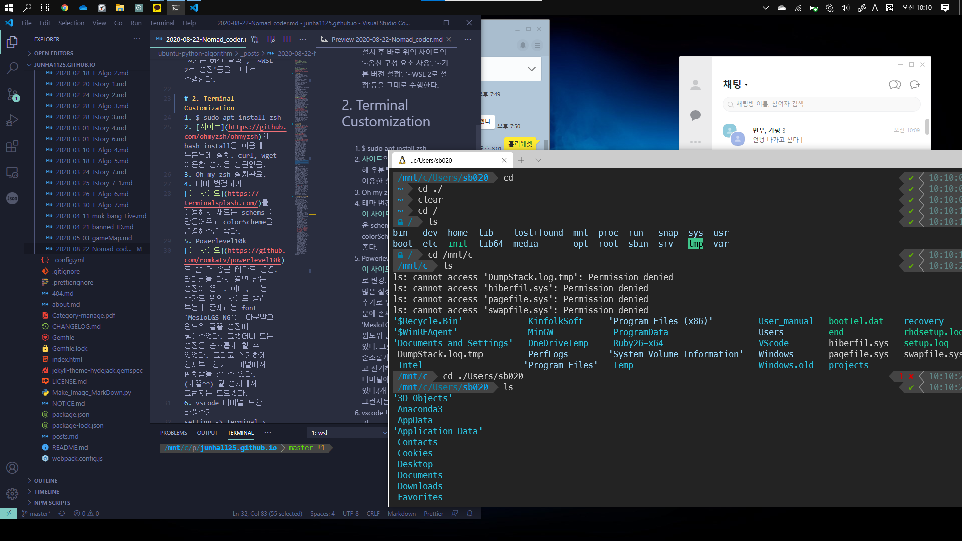
  1. 우분투와 윈도우와의 관계
    $ cd /mnt(mount)/c(c드라이브) -> 우분투와 윈도우를 연결해주는 부분
    $ ls /mnt/c/Users/sb020 -> 결국에 여기가 나의 Document들이 있는 부분
    • 여기서 내가 torch, vi 등으로 파일을 만들고 수정해도 가능하다. 즉 우분투 상에서 윈도우에 접근해서 뭐든 할 수 있는 것이다.
    • 대부분의 WSL사용자들은 우분투 공간에서 윈도우 파일을 만들고 수정하지 않는다. 일반적인 우분투 사용자처럼 /home/junha/~ 에 파일이나 프로젝트를 넣어두고 다룬다. 하지만!! 이러한 방법은 WSL에 문제가 생기거나 Ubuntu-18.04에 문제가 생겨서 지우게 된다면 발생하는 문제를 고스란히 감안해야한다. 따라서 노마드 쌤이 추천하길, 우분투 경로 말고 /mnt/c 위의 윈도우 경로에, 프로젝트 파일 등은 저장하고 다루는 것이 좋다.
    • 리눅스 콘솔에서 윈도우에 있는 파일을 건드릴 수 있다. 하지만 윈도우에서 리눅스 파일(/home/junha 맞나..? 잘 모르곘다. )을 건드린다면 그건 좋은 방법이 아니다. 문제가 발생할 수도 있다.
    • conda에 대한 나의 생각 : zsh의 상태를 보면 conda를 쳐도 읽지를 못한다. 이 말은 conda는 윈도우의 powerShell이나 cmd에서만 동장한다. 따라서 우분투에 들어가서 항상 내가 아나콘다부터 설치한 듯이, 아나콘다를 다시 설치해야한다.^^
  2. bashrc NO!. zshrc Yes!.
    • 강의에서 nodejs를 설치했다. 나는 그동안 anaconda를 설치했다. /home/junha/anaconda에 설치가 되었다. /mnt/c/Users/sb020/anaconda와는 완전히 다른 것이다. 즉 내가 설치한 Ubunutu 18.04에 ubuntu를 설치한 것이고, c드라이브와 영향은 없는 것으로 추측할 수 있다. /ageron/handson-ml/blob/master/requirements.txt) 딥러닝에 유용한 package requirements를 다운받을 수 있었다. (python == 3.6 version이어야 requiremtnet.txt가 잘 작동)
    • 이렇게 처음 설치하면 딥러닝 환경 설정으로 아주 편하다. conda를 사용해서 설정하는게 package 버전 관리에 매우 유용하다. pip을 사용해도 되지만 같이 쓰면 항상 문제가 발생하더라…
        $ conda install Numpy Scipy Scikit-learn Theano TensorFlow Keras PyTorch Pandas Matplotlib      
        $ conda install -c conda-forge opencv  
        $ conda install -c pytorch torchvision
      
    • 엄청난 것을 깨달았다. 왜 ~/.bashrc 에 conda에 관한 아무런 내용이 없지? 라고 생각했다. 왜냐하면 나는 지금 zsh shell을 사용하고 있기 때문이다. 따라서 ~/.zshrc 에 들어가면 conda에 대한 설정이 있었다.
    • vi를 사용해서 파일을 수정할 필요가 이제 없다. $ vi ~/.zshrc 하지말고 $ code ~/.zshrc를 하면 매우 쉽다. (vscode 자동실행) 여기에 들어가서 alias를 이용해서 단축어를 만들어놨다.
        alias python=python3.8  
        alias win="cd /mnt/c/Users/sb020"  
        alias acttor="conda activate torch"  
      
  3. WSL ubuntu VScode
    • image
    • 위의 사진에서 보이는 것처럼, 2가지의 운영체제에서 하나의 vscode를 사용하고 있다. 따라서 Extentions도 여러가지 다시 설치해줘야했다. 또한 VScode 맨아래 왼쪽에 WSL과 Local VScode로 이동할 수 있는 버튼이 있었다.
    • prettier를 사용하면 코드를 save하면 코드를 이쁘게 다 재배열해준다. vscode에 가장 필요한 extentions라고 하는데 진짜인 것 같다. WSL setting에 들어가서 ‘editer format on save’설정을 해줘야한다. 윈도우, 우분투 vscode Setting은 완전히 다르다. 따라서 윈도우도 같은 설정을 해줬다.
    • 하지만… 아래와 같이 이와 같은 오류가 떴다. “Failed to load module. If you have prettier or plugins referenced in package.json, ensure you have run npm install Attempted to load prettier from c:\projects\junha1125.github.io”
    • 그래서 npm 설치하기 위해서 인터넷에서 찾아보니 nodejs를 다운받으라고 해서 choco를 통해 빠르게 다운받았다. 그래도 안됐다.
    • 아래의 사진과 같이 setting도 2가지 환경에서 서로 다르게 셋팅할 수 있으니 주의할 것.
      image
    • 주의 더이상 vi쓰지마라. $ code <pathName or fileName or directoryName>
  4. VScode 사용 주의사항
    • interpretter 설정에 주의하기
      image

【Pytorch 실습】RNN, LSTM을 활용한 영화 평점 예측 모델.

아래의 코드는 Kaggle 및 Git의 공개된 코드를 적극 활용한, 과거의 공부한 내용을 정리한 내용입니다.

【Pytorch 실습】RNN, LSTM을 활용한 영화 리뷰 예측 모델.

  • torchvision이 아니라 torchtext에서 데이터를 가져오기 위해 torchtext import
  • 자연어 같은 경우 Text의 전처리가 가장 중요하다.
  • 자연어를 다뤄야할 일이 있다면 아래의 내용이나 torch document의 내용을 참고 공부하고 공부한다면 더 좋을 것 같다.
import torch
import torch.nn as nn
import torch.nn.functional as F
from torchtext import data, datasets
BATCH_SIZE = 100
LR = 0.001
EPOCHS = 15
USE_CUDA = torch.cuda.is_available()

1. Data Load(Text이므로 어려울 수 있다.)

DEVICE = torch.device("cuda" if USE_CUDA else "cpu")
TEXT = data.Field(sequential = True, batch_first = True, lower = True) # lower : 전부 소문자로
LABEL = data.Field(sequential = False, batch_first = True) # 평점 : 긍정 vs 부정
  • datasets들 중에서 IMDB 데이터를 가져온다. 영화 리뷰 글(Text) + 긍정/부정(Lavel)가 있다.
    trainset, testset = datasets.IMDB.splits(TEXT, LABEL) 
    
  • 데이터가 문장이 되어 있으므로, 띄어쓰기 단위로 단어로 자른다. 그런 후 단어가 총 몇개가 있는지 확인한다. Ex i am a boy = 4 개
    TEXT.build_vocab(trainset, min_freq = 5) # 최고 5번 이상 나온 단어만 voca로 구분하겠다. 
    LABEL.build_vocab(trainset)
    
  • Train dataset과 valuation dataset으로 구분한다. split 함수를 사용하면 쉽다.
  • iter로 놓음으로써, 나중에 베치사이즈 기준으로 학습 시키기 쉽게 만든다.
    trainset, valset = trainset.split(split_ratio = 0.8)
    train_iter, val_iter, test_iter = data.BucketIterator.splits((trainset, valset, testset), batch_size = BATCH_SIZE, shuffle = True, repeat = False)
    
vocab_size = len(TEXT.vocab)
n_classes = 2  # 긍정 vs 부정
print("[TRAIN]: %d \t [VALID]: %d \t [TEST]: %d \t [VOCAB] %d \t [CLASSES] %d" % (len(trainset), len(valset), len(testset), vocab_size, n_classes))

[VOCAB] 46159(Train set안에 있는 voca만) [CLASSES] 2

2. RNN 모델 구현

class BasicRNN(nn.Module):
    def __init__(self, n_layers, hidden_dim, n_vocab, embed_dim, n_classes, dropout_p = 0.2):
        super(BasicRNN, self).__init__()
        print("Building RNN")
        self.n_layers = n_layers # layer 갯수 RNN을 몇번 돌건지
        self.embed = nn.Embedding(n_vocab, embed_dim) # 한 단어를 하나의 백터/값으로 임베팅 한다.
        self.hidden_dim = hidden_dim
        self.dropout = nn.Dropout(dropout_p)
        self.rnn = nn.RNN(embed_dim, self.hidden_dim, num_layers = self.n_layers, batch_first = True) # nn.RNN 을 이용하면 쉽게 RNN구현 가능!!
        self.out = nn.Linear(self.hidden_dim, n_classes) 

    def forward(self, x):
        x = self.embed(x) # 문자를 숫자/백터로 변환
        h_0 = self._init_state(batch_size = x.size(0)) # 가장 첫번째 h0는 아직 정의되지 않았으므로 다음과 같이 정의 해준다. 
        x, _ = self.rnn(x, h_0) # 이렇게 손쉽게 RNN을 구현할 수 있다. 
        h_t = x[:, -1, :] # 모든 문장을 거쳐서 나온 가장 마지막에 나온 단어(평점)의 값
        self.dropout(h_t)
        logit = torch.sigmoid(self.out(h_t))
        return logit

    def _init_state(self, batch_size = 1):
        weight = next(self.parameters()).data # hidden state에 대한 차원은 맞춰주면서 가중치 값은 아직은 0으로 만들어 준다. 
        return weight.new(self.n_layers, batch_size, self.hidden_dim).zero_()

3. 학습 및 추론

def train(model, optimizer, train_iter):
    model.train()
    for b, batch in enumerate(train_iter):
        x, y = batch.text.to(DEVICE), batch.label.to(DEVICE)
        y.data.sub_(1)
        optimizer.zero_grad()

        logit = model(x)
        loss = F.cross_entropy(logit, y)
        loss.backward()
        optimizer.step()

        if b % 50 == 0:
            print("Train Epoch: {} [{}/{} ({:.0f}%)]\tLoss: {:.6f}".format(e,
                                                                           b * len(x),
                                                                           len(train_iter.dataset),
                                                                           100. * b / len(train_iter),
                                                                           loss.item()))
def evaluate(model, val_iter):
    model.eval()
    corrects, total_loss = 0, 0

    for batch in val_iter:
        x, y = batch.text.to(DEVICE), batch.label.to(DEVICE)
        y.data.sub_(1) # 0아니면 1로 데이터 값 수정
        logit = model(x)
        loss = F.cross_entropy(logit, y, reduction = "sum")
        total_loss += loss.item()
        corrects += (logit.max(1)[1].view(y.size()).data == y.data).sum()

    size = len(val_iter.dataset)
    avg_loss = total_loss / size
    avg_accuracy = 100.0 * corrects / size
    return avg_loss, avg_accuracy
model = BasicRNN(n_layers = 1, hidden_dim = 256, n_vocab = vocab_size, embed_dim = 128, n_classes = n_classes, dropout_p = 0.5).to(DEVICE)
optimizer = torch.optim.Adam(model.parameters(), lr = LR)
for e in range(1, EPOCHS + 1):
    train(model, optimizer, train_iter)
    val_loss, val_accuracy = evaluate(model, val_iter)
    print("[EPOCH: %d], Validation Loss: %5.2f | Validation Accuracy: %5.2f" % (e, val_loss, val_accuracy))
Building RNN
Train Epoch: 1 [0/20000 (0%)]	Loss: 0.693486
Train Epoch: 1 [5000/20000 (25%)]	Loss: 0.693027
Train Epoch: 1 [10000/20000 (50%)]	Loss: 0.692615
Train Epoch: 1 [15000/20000 (75%)]	Loss: 0.693534
[EPOCH: 1], Validation Loss:  0.69 | Validation Accuracy: 49.00

Train Epoch: 15 [0/20000 (0%)]	Loss: 0.692949
Train Epoch: 15 [5000/20000 (25%)]	Loss: 0.695515
Train Epoch: 15 [10000/20000 (50%)]	Loss: 0.692522
Train Epoch: 15 [15000/20000 (75%)]	Loss: 0.693040
[EPOCH: 15], Validation Loss:  0.69 | Validation Accuracy: 50.00
test_loss, test_acc = evaluate(model,test_iter)
print("Test Loss: %5.2f | Test Accuracy: %5.2f" % (test_loss, test_acc))
Test Loss:  0.70 | Test Accuracy: 50.00

4. GRU 모델 구현 및 학습추론

  • RNN과 전체적인 구조가 같으나, Hidden state에서 사용되는 gate가 2개이다.
    class BasicGRU(nn.Module):
      def __init__(self, n_layers, hidden_dim, n_vocab, embed_dim, n_classes, dropout_p = 0.2):
          super(BasicGRU, self).__init__()
          print("Building GRU")
          self.n_layers = n_layers
          self.embed = nn.Embedding(n_vocab, embed_dim)
          self.hidden_dim = hidden_dim
          self.dropout = nn.Dropout(dropout_p)
          self.gru = nn.GRU(embed_dim, self.hidden_dim, num_layers = self.n_layers, batch_first = True)
          self.out = nn.Linear(self.hidden_dim, n_classes)
            
      def forward(self, x):
          x = self.embed(x)
          h_0 = self._init_state(batch_size = x.size(0))
          x, _ = self.gru(x, h_0)
          h_t = x[:, -1, :]
          self.dropout(h_t)
          logit = torch.sigmoid(self.out(h_t))
          return logit
        
      def _init_state(self, batch_size = 1):
          weight = next(self.parameters()).data
          return weight.new(self.n_layers, batch_size, self.hidden_dim).zero_()
    
model = BasicGRU(n_layers = 1, hidden_dim = 256, n_vocab = vocab_size, embed_dim = 128, n_classes = n_classes, dropout_p = 0.5).to(DEVICE)
optimizer = torch.optim.Adam(model.parameters(), lr = LR)
for e in range(1, EPOCHS + 1):
    train(model, optimizer, train_iter)
    val_loss, val_accuracy = evaluate(model, val_iter)
    print("[EPOCH: %d], Validation Loss: %5.2f | Validation Accuracy: %5.2f" % (e, val_loss, val_accuracy))
Building GRU
Train Epoch: 1 [0/20000 (0%)]	Loss: 0.691595
Train Epoch: 1 [5000/20000 (25%)]	Loss: 0.693059
Train Epoch: 1 [10000/20000 (50%)]	Loss: 0.693562
Train Epoch: 1 [15000/20000 (75%)]	Loss: 0.693485
[EPOCH: 1], Validation Loss:  0.69 | Validation Accuracy: 50.00
 
Train Epoch: 15 [0/20000 (0%)]	Loss: 0.363591
Train Epoch: 15 [5000/20000 (25%)]	Loss: 0.324579
Train Epoch: 15 [10000/20000 (50%)]	Loss: 0.335097
Train Epoch: 15 [15000/20000 (75%)]	Loss: 0.333244
[EPOCH: 15], Validation Loss:  0.45 | Validation Accuracy: 85.00
test_loss, test_acc = evaluate(model,test_iter)
print("Test Loss: %5.2f | Test Accuracy: %5.2f" % (test_loss, test_acc))
Test Loss:  0.46 | Test Accuracy: 84.00

5. GRU 모델 구현 및 학습추론

  • 알고 있듯이 LSTM의 Cell state의 gate는 forget,input,ouput이 존재한다.
  • 이렇게 nn모듈을 사용해서 LSTM을 쉽게 구현하고 사용할 수 있다.
class BasicLSTM(nn.Module):
    def __init__(self, n_layers, hidden_dim, n_vocab, embed_dim, n_classes, dropout_p = 0.2):
        super(BasicLSTM, self).__init__()
        print("Building LSTM")
        self.n_layers = n_layers
        self.embed = nn.Embedding(n_vocab, embed_dim)
        self.hidden_dim = hidden_dim
        self.dropout = nn.Dropout(dropout_p)
        self.lstm = nn.LSTM(embed_dim, self.hidden_dim, num_layers = self.n_layers, batch_first = True)
        self.out = nn.Linear(self.hidden_dim, n_classes)
        
    def forward(self, x):
        x = self.embed(x)
        h_0 = self._init_state(batch_size = x.size(0))
        c_0 = self._init_state(batch_size = x.size(0))
        
        x, _ = self.lstm(x, (h_0, c_0))
        h_t = x[:, -1, :]
        self.dropout(h_t)
        logit = torch.sigmoid(self.out(h_t))
        return logit
    
    def _init_state(self, batch_size = 1):
        weight = next(self.parameters()).data
        return weight.new(self.n_layers, batch_size, self.hidden_dim).zero_()
model = BasicLSTM(n_layers = 1, hidden_dim = 256, n_vocab = vocab_size, embed_dim = 128, n_classes = n_classes, dropout_p = 0.5).to(DEVICE)
optimizer = torch.optim.Adam(model.parameters(), lr = LR)
for e in range(1, EPOCHS + 1):
    train(model, optimizer, train_iter)
    val_loss, val_accuracy = evaluate(model, val_iter)
    print("[EPOCH: %d], Validation Loss: %5.2f | Validation Accuracy: %5.2f" % (e, val_loss, val_accuracy))
Building LSTM
Train Epoch: 1 [0/20000 (0%)]	Loss: 0.693381
Train Epoch: 1 [5000/20000 (25%)]	Loss: 0.693180
Train Epoch: 1 [10000/20000 (50%)]	Loss: 0.693065
Train Epoch: 1 [15000/20000 (75%)]	Loss: 0.695363
[EPOCH: 1], Validation Loss:  0.69 | Validation Accuracy: 49.00
   
Train Epoch: 15 [0/20000 (0%)]	Loss: 0.427247
Train Epoch: 15 [5000/20000 (25%)]	Loss: 0.454655
Train Epoch: 15 [10000/20000 (50%)]	Loss: 0.428639
Train Epoch: 15 [15000/20000 (75%)]	Loss: 0.428214
[EPOCH: 15], Validation Loss:  0.49 | Validation Accuracy: 82.00
test_loss, test_acc = evaluate(model,test_iter)
print("Test Loss: %5.2f | Test Accuracy: %5.2f" % (test_loss, test_acc))
Test Loss:  0.50 | Test Accuracy: 80.00

【Pytorch 실습】Pytorch 내장 Model 사용, 내장 weight 사용해서 Transfer Learning하기

아래의 코드는 Kaggle 및 Git의 공개된 코드를 적극 활용한, 과거의 공부한 내용을 정리한 내용입니다.

【Pytorch 실습】Pytorch 내장 Model 사용, 내장 weight 사용해서 Transfer Learning하기

1. 데이터 로드

  • 지금까지와는 약간 다르게 데이터 로드
  • hymenoptera_data를 사용할 예정이다. 다운로드 는 여기서 하면 되고, 데이터 구조는 다음과 같다. 꿀벌과 개미를 분류하기 위한 데이터 셋이다.
    image
  • 아래와 같은 방법 전처리 할 수 있다. 지금까지의 dataset, dataloader를 구성할 때와의 방법과는 조금 다르다.
  • 적은 데이터를 이용하기 위해, Data argumentation하는 방법이 아래와 같이 transforms.Compose를 이용하면 되는 것을 알아두자.
import torch 
USE_CUDA = torch.cuda.is_available()
DEVICE = torch.device("cuda" if USE_CUDA else "cpu")
from torchvision import datasets, transforms

data_transforms = {
    'train': transforms.Compose([
        transforms.RandomResizedCrop(224),
        transforms.RandomHorizontalFlip(),
        transforms.ToTensor(),
        transforms.Normalize([0.485, 0.456, 0.406], [0.229, 0.224, 0.225])
    ]),
    'val': transforms.Compose([
        transforms.CenterCrop(224),
        transforms.Resize(256),
        transforms.ToTensor(),
        transforms.Normalize([0.485, 0.456, 0.406], [0.229, 0.224, 0.225])
    ]),
}

image_datasets = {x: datasets.ImageFolder("../data/hymenoptera_data", data_transforms[x]) for x in ['train', 'val']}
dataloaders = {x: torch.utils.data.DataLoader(image_datasets[x], batch_size = 8, num_workers = 0, shuffle = True) for x in ['train', 'val']}
dataset_sizes = {x: len(image_datasets[x]) for x in ['train', 'val']}
class_names = image_datasets['train'].classes

2. 학습 및 추론 함수 정의

def train(model, train_loader, optimizer, epoch):
    model.train()
    for batch_idx, (data, target) in enumerate(train_loader):
        data, target = data.to(DEVICE), target.to(DEVICE)
        optimizer.zero_grad()
        output = model(data)
        loss = F.cross_entropy(output, target)
        loss.backward()
        optimizer.step()
        
        if batch_idx % 10 == 0:
            print("Train Epoch: {} [{}/{} ({:.0f}%)]\tLoss: {:.6f}".format(
                epoch, 
                batch_idx * len(data), 
                len(train_loader.dataset), 
                100. * batch_idx / len(train_loader), 
                loss.item()))


def evaluate(model, test_loader):
    model.eval()
    test_loss = 0
    correct = 0
    with torch.no_grad():
        for data, target in test_loader:
            data, target = data.to(DEVICE), target.to(DEVICE)
            output = model(data)
            test_loss += F.cross_entropy(output, target, reduction = "sum").item()
            prediction = output.max(1, keepdim = True)[1]
            correct += prediction.eq(target.view_as(prediction)).sum().item()
    
    test_loss /= len(test_loader.dataset)
    test_accuracy = 100. * correct / len(test_loader.dataset)
    return test_loss, test_accuracy

3. 내장 모델 사용하기(Transfer Learning 안함)

  • pretrained = True 를 사용하면 ImageNet에서 사용한 파라메터를 사용한다.
  • torch의 내장 모델을 그냥 사용할 때, input과 output사이즈(Groud True data size)는 현재 나의 data에 따라서 달라지기 떄문에 전혀 걱정하지 않아도 된다.
import torchvision.models as models
import torch.nn as nn
import torch.optim as optim
import torch.nn.functional as F

model = models.resnet18(pretrained = False).cuda()
optimizer = optim.Adam(model.parameters(), lr = 0.0001)
EPOCHS = 10
for epoch in range(1, EPOCHS + 1):
    train(model, dataloaders["train"], optimizer, epoch)
    test_loss, test_accuracy = evaluate(model, dataloaders["val"])
    print("[{}] Test Loss: {:.4f}, accuracy: {:.2f}%\n".format(epoch, test_loss, test_accuracy))
Train Epoch: 10 [0/397 (0%)]	Loss: 0.636741
Train Epoch: 10 [80/397 (20%)]	Loss: 0.449106
Train Epoch: 10 [160/397 (40%)]	Loss: 0.607533
Train Epoch: 10 [240/397 (60%)]	Loss: 0.713035
Train Epoch: 10 [320/397 (80%)]	Loss: 0.705570
[10] Test Loss: 0.6319, accuracy: 66.25%

4. 내장 모델 사용하기(Transfer Learning 사용)

  • pretrained된 weight를 사용하면, 마지막 Feature는 1*1000(ImageNet의 Class 갯수)이다.
  • 따라서 마지막에 출력되는 Feature의 갯수를 지금 나의 데이터의 Class의 갯수로 맞춰줘야 한다. 따라서 다음과 같은 작업을 수행한다.
model = models.resnet18(pretrained = True) 
num_ftrs = model.fc.in_features   # fully connected layer에 들어가기 직전의 feature의 갯수(numbers)를 알아온다. 
model.fc = nn.Linear(num_ftrs, 2) 
# model의 마지막 fully connected layer의 정의를 바꿔 버린다.  
model.fc = nn.Linear(num_ftrs, 2) 
# 원래는 num_ftrs -> 1000 이었다면, num_ftrs -> 2 으로 바꾼다. 


if USE_CUDA:
    model = model.cuda()

optimizer = optim.Adam(model.parameters(), lr = 0.0001)
EPOCHS = 10
for epoch in range(1, EPOCHS + 1):
    train(model, dataloaders["train"], optimizer, epoch)
    test_loss, test_accuracy = evaluate(model, dataloaders["val"])
    print("[{}] Test Loss: {:.4f}, accuracy: {:.2f}%\n".format(epoch, test_loss, test_accuracy))
Train Epoch: 10 [0/397 (0%)]	Loss: 0.821322
Train Epoch: 10 [80/397 (20%)]	Loss: 0.526726
Train Epoch: 10 [160/397 (40%)]	Loss: 0.820258
Train Epoch: 10 [240/397 (60%)]	Loss: 0.242522
Train Epoch: 10 [320/397 (80%)]	Loss: 0.604658
[10] Test Loss: 0.2158, accuracy: 93.70%
  • param.requires_grad = False : Backward에 의해서 gradient 계산이 안된다.
  • 아래와 같이 코딩을 하면 ‘nn.Linear(num_ftrs, 2)’로 정의한 마지막 Layer만 Backpropagation으로 weight가 update되지만, 나머지 pretrained weight 즉 가져온 weight는 변하지 않는다.
model = models.resnet18(pretrained=True)
for param in model.parameters():
    param.requires_grad = False 
num_ftrs = model.fc.in_features
model.fc = nn.Linear(num_ftrs, 2)

model = model.cuda()

optimizer = optim.Adam(model.parameters(), lr = 0.0001)

EPOCHS = 10
for epoch in range(1, EPOCHS + 1):
    train(model, dataloaders["train"], optimizer, epoch)
    test_loss, test_accuracy = evaluate(model, dataloaders["val"])
    print("[{}] Test Loss: {:.4f}, accuracy: {:.2f}%\n".format(epoch, test_loss, test_accuracy))
Train Epoch: 10 [0/397 (0%)]	Loss: 0.773592
Train Epoch: 10 [80/397 (20%)]	Loss: 0.575552
Train Epoch: 10 [160/397 (40%)]	Loss: 0.498209
Train Epoch: 10 [240/397 (60%)]	Loss: 0.761115
Train Epoch: 10 [320/397 (80%)]	Loss: 0.598199
[10] Test Loss: 0.6826, accuracy: 59.45%

【Pytorch 실습】 CIFAR10 데이터셋. Dropout, Xivier Weight + ResNet18 사용하기

아래의 코드는 Kaggle 및 Git의 공개된 코드를 적극 활용한, 과거의 공부한 내용을 정리한 내용입니다.

【Pytorch 실습】 CIFAR10 데이터셋. Dropout, Xivier Weight + ResNet18 사용하기

1. Dropout 사용해보기

1. 데이터 Load

import torch
USE_CUDA = torch.cuda.is_available()
DEVICE = torch.device("cuda" if USE_CUDA else "cpu")
  • 공개적인 데이터를 다음과 같이 datasets.~~ 해보면 정말 많은 데이터가 있는 것을 확인할 수 있다.
  • Trainsforms.compose를 이용해서 Tensor형으로 바꿔주는 전처리를 해줄 수 있다.
  • Normalize(평균, 분산) -> RGV에 대해서 정규처리를 해줄 수 있다. ```python from torchvision import transforms, datasets train_loader = torch.utils.data.DataLoader( datasets.CIFAR10(“../data/CIFAR_10/”, train = True, download = True, transform = transforms.Compose([ transforms.RandomHorizontalFlip(), transforms.ToTensor(), transforms.Normalize((0.5, 0.5, 0.5), (0.5, 0.5, 0.5))])), batch_size = 64, shuffle = True)

test_loader = torch.utils.data.DataLoader( datasets.CIFAR10(“../data/CIFAR_10”, train = False, transform = transforms.Compose([ transforms.RandomHorizontalFlip(), transforms.ToTensor(), transforms.Normalize((0.5, 0.5, 0.5), (0.5, 0.5, 0.5))])), batch_size = 64 )


## 2. 모델 구현
- 드롭아웃을 하는 방법은 아래와 같다. 여기서는 Fully Connected layer에서 dropout을 사용했는데, 내부 동작원리는 간단하다. 
- layer의 node 중 랜덤하게 일정비율로 0으로 만들어 버리는 것이다. (node가 동작하지 않는다.) 이렇게 함으로써 간단하게 dropout을 구현할 수 있다. 
- 아래에서 사용한 변수 self.dropout_o = 0.2가 랜덤하게 노드를 잠그는 비율이다. 

```python
import torch.nn as nn
import torch.nn.functional as F
import torch.optim as optim
    
class CNN(nn.Module):
    def __init__(self):
        super(CNN, self).__init__()
        self.conv1 = nn.Conv2d(in_channels = 3, out_channels = 8, kernel_size = 3, padding = 1)
        self.conv2 = nn.Conv2d(in_channels = 8, out_channels = 16, kernel_size = 3, padding = 1)
        self.conv3 = nn.Conv2d(in_channels = 16, out_channels = 32, kernel_size = 3, padding = 1)
        self.conv4 = nn.Conv2d(in_channels = 32, out_channels = 64, kernel_size = 3, padding = 1)
        self.pool = nn.MaxPool2d(kernel_size = 2, stride = 2)
        self.fc1 = nn.Linear(2 * 2 * 64, 64)
        self.fc2 = nn.Linear(64, 32)
        self.fc3 = nn.Linear(32, 10)
        
        self.conv1_bn = nn.BatchNorm2d(8)
        self.conv2_bn = nn.BatchNorm2d(16)
        self.conv3_bn = nn.BatchNorm2d(32)
        self.conv4_bn = nn.BatchNorm2d(64)
        
        self.dropout_p = 0.2  # dropout 확률 
        
    def forward(self, x):
        x = self.conv1(x) # 32 * 32 * 3 -> 32 * 32 * 8
        x = self.conv1_bn(x)
        x = F.tanh(x)     # 32 * 32 * 8
        x = self.pool(x)  # 16 * 16 * 8
        
        x = self.conv2(x) # 16 * 16 * 8 -> 16 * 16 * 16
        x = self.conv2_bn(x)
        x = F.tanh(x)     # 16 * 16 * 16
        x = self.pool(x)  # 8  *  8 * 16
        
        x = self.conv3(x) # 8 * 8 * 16 -> 8 * 8 * 32
        x = self.conv3_bn(x)
        x = F.tanh(x)     # 8 * 8 * 32
        x = self.pool(x)  # 4 * 4 * 32
        
        x = self.conv4(x) # 4 * 4 * 32 -> 4 * 4 * 64
        x = self.conv4_bn(x)
        x = F.tanh(x)     # 4 * 4 * 64
        x = self.pool(x)  # 2 * 2 * 64
        
        x = x.view(-1, 2 * 2 * 64)
        x = self.fc1(x)
        x = F.dropout(x, p = self.dropout_p)  # actiavtion function 전후 상관 없다. 알아서..
        x = F.relu(x)
        x = self.fc2(x)
        x = F.dropout(x, p = self.dropout_p)
        x = F.relu(x)
        x = self.fc3(x)
        x = F.log_softmax(x, dim = 1)
        return x

print("DEVICE: ", DEVICE)
print("MODEL: ", model)

DEVICE:  cuda
MODEL:  CNN(
  (conv1): Conv2d(3, 8, kernel_size=(3, 3), stride=(1, 1), padding=(1, 1))
  (conv2): Conv2d(8, 16, kernel_size=(3, 3), stride=(1, 1), padding=(1, 1))
  (conv3): Conv2d(16, 32, kernel_size=(3, 3), stride=(1, 1), padding=(1, 1))
  (conv4): Conv2d(32, 64, kernel_size=(3, 3), stride=(1, 1), padding=(1, 1))
  (pool): MaxPool2d(kernel_size=2, stride=2, padding=0, dilation=1, ceil_mode=False)
  (fc1): Linear(in_features=256, out_features=64, bias=True)
  (fc2): Linear(in_features=64, out_features=32, bias=True)
  (fc3): Linear(in_features=32, out_features=10, bias=True)
  (conv1_bn): BatchNorm2d(8, eps=1e-05, momentum=0.1, affine=True, track_running_stats=True)
  (conv2_bn): BatchNorm2d(16, eps=1e-05, momentum=0.1, affine=True, track_running_stats=True)
  (conv3_bn): BatchNorm2d(32, eps=1e-05, momentum=0.1, affine=True, track_running_stats=True)
  (conv4_bn): BatchNorm2d(64, eps=1e-05, momentum=0.1, affine=True, track_running_stats=True)
)

3. 가중치 초기화 하기

  • 보통은 Transfer Learning을 통해서 가중치 초기화에 대해서 공부할 기회가 없지만 여기서는 가중치 초기화를 직접 해보았다.
  • 가중치를 초기화 하는 방법에는 Xavier와 He등이 있다. 여기서는 Xavier를 사용해 보았다. Relu를 사용한 모델에서는 He를 사용하는게 더 유리하다고 하다.
    ```python

import torch.nn.init as init def weight_init(m):

'''
이 주석을 풀면 Xavier, kaiming 에 대한 Initialization에 대한 상세 설정을 할 수 있다. 

Ref: https://pytorch.org/docs/stable/nn.init.html

init.uniform_(tensor, a = 0.0, b = 1.0) (a: Lower bound, b: Upper bound)
init.normal_(tensor, mean = 0.0, std = 1.0)
init.xavier_uniform_(tensor, gain = 1.0)
init.xavier_normal_(tensor, gain = 1.0)
init.kaiming_uniform_(tensor, a=0, mode='fan_in', nonlinearity='leaky_relu')
init.kaiming_normal_(tensor, a=0, mode='fan_in', nonlinearity='leaky_relu')
'''

if isinstance(m, nn.Conv2d):
    init.xavier_uniform_(m.weight.data)
    if m.bias is not None:
        init.normal_(m.bias.data)

elif isinstance(m, nn.BatchNorm2d):
    init.normal_(m.weight.data, mean=1, std=0.02)
    init.constant_(m.bias.data, 0)

elif isinstance(m, nn.Linear):
    init.xavier_uniform_(m.weight.data)
    init.normal_(m.bias.data)

model = CNN().to(DEVICE) model.apply(weight_init)

optimizer = optim.Adam(model.parameters(), lr = 0.001) print(“DEVICE: “, DEVICE) print(“MODEL: “, model)


## 4. 모델 학습 및 추론
```python
def train(model, train_loader, optimizer, epoch):
    model.train()
    for batch_idx, (data, target) in enumerate(train_loader):
        data, target = data.to(DEVICE), target.to(DEVICE)
        optimizer.zero_grad()
        output = model(data)
        loss = F.cross_entropy(output, target)
        loss.backward()
        optimizer.step()
        
        if batch_idx % 100 == 0:
            print("Train Epoch: {} [{}/{} ({:.0f}%)]\tLoss: {:.6f}".format(
                epoch, 
                batch_idx * len(data), 
                len(train_loader.dataset), 
                100. * batch_idx / len(train_loader), 
                loss.item()))
def evaluate(model, test_loader):
    model.eval()
    test_loss = 0
    correct = 0
    with torch.no_grad():
        for data, target in test_loader:
            data, target = data.to(DEVICE), target.to(DEVICE)
            output = model(data)
            test_loss += F.cross_entropy(output, target, reduction = "sum").item()
            prediction = output.max(1, keepdim = True)[1]
            correct += prediction.eq(target.view_as(prediction)).sum().item()
    
    test_loss /= len(test_loader.dataset)
    test_accuracy = 100. * correct / len(test_loader.dataset)
    return test_loss, test_accuracy
EPOCHS = 10
for epoch in range(1, EPOCHS + 1):
    train(model, train_loader, optimizer, epoch)
    test_loss, test_accuracy = evaluate(model, test_loader)
    print("[{}] Test Loss: {:.4f}, accuracy: {:.2f}%\n".format(epoch, test_loss, test_accuracy))
Train Epoch: 10 [0/50000 (0%)]	Loss: 1.137886
Train Epoch: 10 [6400/50000 (13%)]	Loss: 0.988332
Train Epoch: 10 [12800/50000 (26%)]	Loss: 0.784159
Train Epoch: 10 [19200/50000 (38%)]	Loss: 1.073874
Train Epoch: 10 [25600/50000 (51%)]	Loss: 1.101201
Train Epoch: 10 [32000/50000 (64%)]	Loss: 1.111024
Train Epoch: 10 [38400/50000 (77%)]	Loss: 0.956936
Train Epoch: 10 [44800/50000 (90%)]	Loss: 0.914141
[10] Test Loss: 1.0315, accuracy: 64.86%
print("CNN's number of Parameters: ", sum([p.numel() for p in model.parameters()]))
CNN's number of Parameters:  43626

2. ResNet 사용해보기

1. 데이터 Load

import torch
USE_CUDA = torch.cuda.is_available()
DEVICE = torch.device("cuda" if USE_CUDA else "cpu")
from torchvision import transforms, datasets
train_loader = torch.utils.data.DataLoader(
    datasets.CIFAR10("../data/CIFAR_10/",
                     train = True,
                     download = True,
                     transform = transforms.Compose([
                         transforms.RandomHorizontalFlip(),
                         transforms.ToTensor(),
                         transforms.Normalize((0.5, 0.5, 0.5),
                                              (0.5, 0.5, 0.5))])), batch_size = 64, shuffle = True)

test_loader = torch.utils.data.DataLoader(
    datasets.CIFAR10("../data/CIFAR_10",
                     train = False,
                     transform = transforms.Compose([
                         transforms.RandomHorizontalFlip(),
                         transforms.ToTensor(),
                         transforms.Normalize((0.5, 0.5, 0.5),
                                              (0.5, 0.5, 0.5))])), batch_size = 64 , shuffle = True)

2. ResNet 모델 구현하기

import torch.nn as nn
import torch.nn.functional as F
import torch.optim as optim

class BasicBlock(nn.Module): # bottlenexk 이라는 용어로도 많이 사용된다.
    def __init__(self, in_planes, planes, stride = 1):
        super(BasicBlock, self).__init__()
        self.conv1 = nn.Conv2d(in_planes, planes, kernel_size = 3, stride = stride, padding = 1, bias = False)
        self.bn1 = nn.BatchNorm2d(planes)
        self.conv2 = nn.Conv2d(planes, planes, kernel_size = 3, stride = 1, padding = 1, bias = False)
        self.bn2 = nn.BatchNorm2d(planes)
        
        self.shortcut = nn.Sequential()
        if stride != 1 or in_planes != planes:
            self.shortcut = nn.Sequential(
                nn.Conv2d(in_planes, planes, kernel_size = 1, stride = stride, bias = False),
                nn.BatchNorm2d(planes))
    
    def forward(self, x):
        out = F.relu(self.bn1(self.conv1(x)))
        out = self.bn2(self.conv2(out))
        out += self.shortcut(x)
        out = F.relu(out)
        return out
    
class ResNet(nn.Module): # _ㄴmake_layer라는 용어로 많이 사용되니, 알아두기
    def __init__(self, num_classes = 10):
        super(ResNet, self).__init__()
        self.in_planes = 16
        
        self.conv1 = nn.Conv2d(3, 16, kernel_size = 3, stride = 1, padding = 1, bias = False)
        self.bn1 = nn.BatchNorm2d(16)
        self.layer1 = self._make_layer(16, 2, stride = 1)
        self.layer2 = self._make_layer(32, 2, stride = 2)
        self.layer3 = self._make_layer(64, 2, stride = 2)
        self.linear = nn.Linear(64, num_classes)
        
    def _make_layer(self, planes, num_blocks, stride):
        strides = [stride] + [1] * (num_blocks  - 1)
        layers = []
        for stride in strides:
            layers.append(BasicBlock(self.in_planes, planes, stride))
            self.in_planes = planes
        return nn.Sequential(*layers)
    
    def forward(self, x):
        out = F.relu(self.bn1(self.conv1(x)))
        out = self.layer1(out)
        out = self.layer2(out)
        out = self.layer3(out)
        out = F.avg_pool2d(out, 8)
        out = out.view(out.size(0), -1)
        out = self.linear(out)
        return out
model = ResNet().to(DEVICE)
optimizer = optim.Adam(model.parameters(), lr = 0.001)

print("DEVICE: ", DEVICE)
print("MODEL: ", model)

3. 학습 및 추론

def train(model, train_loader, optimizer, epoch):
    model.train()
    for batch_idx, (data, target) in enumerate(train_loader):
        data, target = data.to(DEVICE), target.to(DEVICE)
        optimizer.zero_grad()
        output = model(data)
        loss = F.cross_entropy(output, target)
        loss.backward()
        optimizer.step()
        
        if batch_idx % 100 == 0:
            print("Train Epoch: {} [{}/{} ({:.0f}%)]\tLoss: {:.6f}".format(
                epoch, 
                batch_idx * len(data), 
                len(train_loader.dataset), 
                100. * batch_idx / len(train_loader), 
                loss.item()))
def evaluate(model, test_loader):
    model.eval()
    test_loss = 0
    correct = 0
    with torch.no_grad():
        for data, target in test_loader:
            data, target = data.to(DEVICE), target.to(DEVICE)
            output = model(data)
            test_loss += F.cross_entropy(output, target, reduction = "sum").item()
            prediction = output.max(1, keepdim = True)[1]
            correct += prediction.eq(target.view_as(prediction)).sum().item()
    
    test_loss /= len(test_loader.dataset)
    test_accuracy = 100. * correct / len(test_loader.dataset)
    return test_loss, test_accuracy
EPOCHS = 3
for epoch in range(1, EPOCHS + 1):
    train(model, train_loader, optimizer, epoch)
    test_loss, test_accuracy = evaluate(model, test_loader)
    print("[{}] Test Loss: {:.4f}, accuracy: {:.2f}%\n".format(epoch, test_loss, test_accuracy))
Train Epoch: 3 [0/50000 (0%)]	Loss: 1.127532
Train Epoch: 3 [6400/50000 (13%)]	Loss: 1.081882
Train Epoch: 3 [12800/50000 (26%)]	Loss: 0.691810
Train Epoch: 3 [19200/50000 (38%)]	Loss: 0.759505
Train Epoch: 3 [25600/50000 (51%)]	Loss: 0.786468
Train Epoch: 3 [32000/50000 (64%)]	Loss: 0.904780
Train Epoch: 3 [38400/50000 (77%)]	Loss: 0.772286
Train Epoch: 3 [44800/50000 (90%)]	Loss: 0.593489
[3] Test Loss: 0.7578, accuracy: 73.14%

3. 유명한 모델 그대로 가져와 사용하는 방법

  • 기본적으로 Pytorch에 저장되어 있는 모델 사용하기.
  • 아래와 같이 굳이 모델을 위에 처럼 구현하지 않아도 아래처럼 쉽게, 학습시킬 수 있다.
import torchvision.models as models
model = models.resnet18().cuda()
optimizer = optim.Adam(model.parameters(), lr = 0.001)
EPOCHS = 3
for epoch in range(1, EPOCHS + 1):
    train(model, train_loader, optimizer, epoch)
    test_loss, test_accuracy = evaluate(model, test_loader)
    print("[{}] Test Loss: {:.4f}, accuracy: {:.2f}%\n".format(epoch, test_loss, test_accuracy))
Train Epoch: 3 [0/50000 (0%)]	Loss: 0.853458
Train Epoch: 3 [6400/50000 (13%)]	Loss: 0.816588
Train Epoch: 3 [12800/50000 (26%)]	Loss: 0.678977
Train Epoch: 3 [19200/50000 (38%)]	Loss: 0.873804
Train Epoch: 3 [25600/50000 (51%)]	Loss: 0.783468
Train Epoch: 3 [32000/50000 (64%)]	Loss: 1.123129
Train Epoch: 3 [38400/50000 (77%)]	Loss: 0.890110
Train Epoch: 3 [44800/50000 (90%)]	Loss: 0.780257
[3] Test Loss: 0.8566, accuracy: 70.31%

resnet18 = models.resnet18()
alexnet = models.alexnet()
vgg16 = models.vgg16()
squeezenet = models.squeezenet1_0()
densenet = models.densenet161()
inception = models.inception_v3()
googlenet = models.googlenet()
shufflenet = models.shufflenet_v2_x1_0()
mobilenet = models.mobilenet_v2()
resnext50_32x4d = models.resnext50_32x4d()
wide_resnet50_2 = models.wide_resnet50_2()
mnasnet = models.mnasnet1_0()

【Pytorch 실습】 CIFAR10 데이터셋. 학습 및 추론, Activation fucntion = relu, tanh

아래의 코드는 Kaggle 및 Git의 공개된 코드를 적극 활용한, 과거의 공부한 내용을 정리한 내용입니다.

  • 코드를 한줄한줄 치면서 공부해보기로 했다. CIRAR10 데이터를 사용해서 모델을 학습시키고 추론해보는 일렬의 과정들을 공부해보자. 그리고 Python과 모델 구현을 잘하는 방법은 눈으로 공부하는 것도 있지만, 한줄한줄 코드를 치면서 공부하고 깨닫는 것이 매우 중요하다고 하다.
  • 데이터셋 다운로드 : https://www.cs.toronto.edu/~kriz/cifar.html
  • 이번 Post의 목적은 코드를 한줄한줄 치면서 어떻게 공부하고 검색하는지에 대한 느낌을 가져가는 것이다.

1. Activation Function : Relu

1. 데이터 Load, 분할(train,valu), Pytorch.tensor.Load

def unpickle(file):
    import pickle
    with open(file, "rb") as fo:
        dict = pickle.load(fo, encoding = "bytes")
    return dict

다운 받은 파일에 1. data_batch1,2,3,4,5, 2. test 파일이 있다. 당연히 전자는 Train데이터 들이다.

tmp = unpickle("../data/CIFAR10/cifar-10-batches-py/data_batch_1")
# 이런식으로 변수를 계속 print해보고 확인해보면, 사실 다 별거아니다. 
print(tmp.keys())
tmp[b'data'].shape
(10000, 3072)
# 위의 일렬의 과정을 data_batch_1,2,3,4,5를 모두 해야하기 때문에 함수로 정의해 사용.
def pickle_to_images_and_labels(root):
    data = unpickle(root)
    data_images = data[b'data'] / 255
    data_images = data_images.reshape(-1, 3, 32, 32).astype("float32")
    data_labels = data[b'labels']
    return data_images, data_labels
images1, label1 = pickle_to_images_and_labels("../data/CIFAR10/cifar-10-batches-py/data_batch_1")
images2, label2 = pickle_to_images_and_labels("../data/CIFAR10/cifar-10-batches-py/data_batch_2")
images3, label3 = pickle_to_images_and_labels("../data/CIFAR10/cifar-10-batches-py/data_batch_3")
images4, label4 = pickle_to_images_and_labels("../data/CIFAR10/cifar-10-batches-py/data_batch_4")
images5, label5 = pickle_to_images_and_labels("../data/CIFAR10/cifar-10-batches-py/data_batch_5")
test_images, test_labels = pickle_to_images_and_labels("../data/CIFAR10/cifar-10-batches-py/test_batch")

아하.. 분할되어 다운받은 이미지 어떻게 할지 궁금했는데, 걍 Concatenation 해버리네…?? 이렇게 데이터가 분할되어 있으면 일단 가져오고, Concatenation해버리면 되는구나 라고 알아두자.

import numpy as np
train_images = np.concatenate([images1, images2, images3, images4, images5], axis = 0)
train_labels = np.concatenate([label1, label2, label3, label4, label5], axis = 0)
test_images = np.concatenate([test_images], axis = 0)
test_labels = np.concatenate([test_labels], axis = 0)
from sklearn.model_selection import train_test_split
train_images, valid_images, train_labels, valid_labels = train_test_split(train_images, train_labels, stratify = train_labels, random_state = 42, test_size = 0.2)
print("The Shape of Train Images: ", train_images.shape)
print("The Shape of Valid Images: ", valid_images.shape)
print("The Shape of Test Images: ", test_images.shape)
The Shape of Train Images:  (40000, 3, 32, 32)
The Shape of Valid Images:  (10000, 3, 32, 32)
The Shape of Test Images:  (10000, 3, 32, 32)
print("The number of Train Labels: ", train_labels.shape)
print("The number of Valid Labels: ", valid_labels.shape)
print("The number of Test Labels: ", test_labels.shape)
The number of Train Labels:  (40000,)
The number of Valid Labels:  (10000,)
The number of Test Labels:  (10000,)
import torch
from torch.utils.data import TensorDataset, DataLoader
train_images_tensor = torch.tensor(train_images)
train_labels_tensor = torch.tensor(train_labels)
train_tensor = TensorDataset(train_images_tensor, train_labels_tensor)
train_loader = DataLoader(train_tensor, batch_size = 64, num_workers = 0, shuffle = True)

valid_images_tensor = torch.tensor(valid_images)
valid_labels_tensor = torch.tensor(valid_labels)
valid_tensor = TensorDataset(valid_images_tensor, valid_labels_tensor)
valid_loader = DataLoader(valid_tensor, batch_size = 64, num_workers = 0, shuffle = True)

test_images_tensor = torch.tensor(test_images)

2. 모델 구현

import torch.nn as nn
import torch.nn.functional as F
import torch.optim as optim

class CNN(nn.Module):
    def __init__(self):
        super(CNN, self).__init__()
        self.conv1 = nn.Conv2d(in_channels = 3, out_channels = 8, kernel_size = 3, padding = 1)
        self.conv2 = nn.Conv2d(in_channels = 8, out_channels = 16, kernel_size = 3, padding = 1)
        self.pool = nn.MaxPool2d(kernel_size = 2, stride = 2)
        self.fc1 = nn.Linear(8 * 8 * 16, 64)
        self.fc2 = nn.Linear(64, 32)
        self.fc3 = nn.Linear(32, 10)
        
    def forward(self, x):
        x = self.conv1(x) # 32 * 32 * 8
        x = F.relu(x)     # 32 * 32 * 8
        x = self.pool(x)  # 16 * 16 * 8
        x = self.conv2(x) # 16 * 16 * 16
        x = F.relu(x)     # 16 * 16 * 16
        x = self.pool(x)  # 8 * 8 * 16
        
        x = x.view(-1, 8 * 8 * 16)
        x = self.fc1(x)
        x = F.relu(x)
        x = self.fc2(x)
        x = F.relu(x)
        x = self.fc3(x)
        x = F.log_softmax(x)
        return x
USE_CUDA = torch.cuda.is_available()
DEVICE = torch.device("cuda" if USE_CUDA else "cpu")
model = CNN().to(DEVICE)
optimizer = optim.Adam(model.parameters(), lr = 0.001)
print("Model: ", model)
print("Device: ", DEVICE)
Model:  CNN(
  (conv1): Conv2d(3, 8, kernel_size=(3, 3), stride=(1, 1), padding=(1, 1))
  (conv2): Conv2d(8, 16, kernel_size=(3, 3), stride=(1, 1), padding=(1, 1))
  (pool): MaxPool2d(kernel_size=2, stride=2, padding=0, dilation=1, ceil_mode=False)
  (fc1): Linear(in_features=1024, out_features=64, bias=True)
  (fc2): Linear(in_features=64, out_features=32, bias=True)
  (fc3): Linear(in_features=32, out_features=10, bias=True)
)
Device:  cuda

3. 학습 및 추론

def train(model, train_loader, optimizer):
    model.train()
    for batch_idx, (data, target) in enumerate(train_loader):
        data, target = data.to(DEVICE), target.to(DEVICE, dtype = torch.int64)
        optimizer.zero_grad()
        output = model(data)
        loss = F.cross_entropy(output, target)
        loss.backward()
        optimizer.step()
        
        if batch_idx % 100 == 0:
            print("Train Epoch: {} [{}/{} ({:.0f}%)]\tLoss: {:.6f}".format(
            epoch, batch_idx * len(data), len(train_loader.dataset), 100. * batch_idx / len(train_loader), loss.item()))
def evaluate(model, valid_loader):
    model.eval()
    
    valid_loss = 0
    correct = 0
    
    with torch.no_grad():
        for data, target in valid_loader:
            data, target= data.to(DEVICE), target.to(DEVICE, dtype = torch.int64)
            output = model(data)
            valid_loss += F.cross_entropy(output, target, reduction = "sum").item()
            prediction = output.max(1, keepdim = True)[1]  # 예측한 class score 중 가장 큰 index 어딘지? 즉 Class가 무엇인지. 
            correct += prediction.eq(target.view_as(prediction)).sum().item() # Ground True와 예측한 값이 몇개인지 계산해서 정확도를 파악한다. 
    
    valid_loss /= len(valid_loader.dataset)
    valid_accuracy = 100. * correct / len(valid_loader.dataset)
    return valid_loss, valid_accuracy
'''TRAINING'''
EPOCHS = 10
for epoch in range(1, EPOCHS + 1):
    train(model, train_loader, optimizer)
    valid_loss, valid_accuracy = evaluate(model, valid_loader)
    print("[EPOCH : {}], \tValidation Loss: {:.4f}, \tValidation Accuracy: {:.2f} % \n".format(
        epoch, valid_loss, valid_accuracy))
Train Epoch: 9 [0/40000 (0%)]	Loss: 1.180444
Train Epoch: 9 [6400/40000 (16%)]	Loss: 1.049773
Train Epoch: 9 [12800/40000 (32%)]	Loss: 0.980881
Train Epoch: 9 [19200/40000 (48%)]	Loss: 1.017157
Train Epoch: 9 [25600/40000 (64%)]	Loss: 0.960528
Train Epoch: 9 [32000/40000 (80%)]	Loss: 1.220239
Train Epoch: 9 [38400/40000 (96%)]	Loss: 0.947019
[EPOCH : 9], 	Validation Loss: 1.1328, 	Validation Accuracy: 60.19 % 

Train Epoch: 10 [0/40000 (0%)]	Loss: 0.898633
Train Epoch: 10 [6400/40000 (16%)]	Loss: 1.141634
Train Epoch: 10 [12800/40000 (32%)]	Loss: 0.852636
Train Epoch: 10 [19200/40000 (48%)]	Loss: 1.075439
Train Epoch: 10 [25600/40000 (64%)]	Loss: 1.237481
Train Epoch: 10 [32000/40000 (80%)]	Loss: 1.139879
Train Epoch: 10 [38400/40000 (96%)]	Loss: 0.973299
[EPOCH : 10], 	Validation Loss: 1.1565, 	Validation Accuracy: 58.96 % 

4. 추론 및 테스트 출력해보기

def testset_prediction(model, test_images_tensor):
    model.eval()
    result = []
    
    with torch.no_grad():
        for data in test_images_tensor:
            data = data.to(DEVICE)
            output = model(data.view(-1, 3, 32, 32))
            prediction = output.max(1, keepdim = True)[1]
            result.append(prediction.tolist())
    return result
from sklearn.metrics import accuracy_score
test_predict_result = testset_prediction(model, test_images_tensor)
accuracy_score(test_labels, np.squeeze(test_predict_result))
0.5898
test_images[30].shape
(3, 32, 32)
import matplotlib.pyplot as plt
plt.imshow(np.transpose(test_images[30], (1, 2, 0)))
plt.show()
test_labels[30]
6
test_predict_result[30]
[[6]]


2. Activation Function : tanh

코드 전계 과정은 위와 동일

import torch
USE_CUDA = torch.cuda.is_available()
DEVICE = torch.device("cuda" if USE_CUDA else "cpu")
from torchvision import transforms, datasets
train_loader = torch.utils.data.DataLoader(
    datasets.CIFAR10("../data/CIFAR_10/",
                     train = True,
                     download = True,
                     transform = transforms.Compose([
                         transforms.RandomHorizontalFlip(),
                         transforms.ToTensor(),
                         transforms.Normalize((0.5, 0.5, 0.5),
                                              (0.5, 0.5, 0.5))])), batch_size = 64, shuffle = True)

test_loader = torch.utils.data.DataLoader(
    datasets.CIFAR10("../data/CIFAR_10",
                     train = False,
                     transform = transforms.Compose([
                         transforms.RandomHorizontalFlip(),
                         transforms.ToTensor(),
                         transforms.Normalize((0.5, 0.5, 0.5),
                                              (0.5, 0.5, 0.5))])), batch_size = 64)
import torch.nn as nn
import torch.nn.functional as F
import torch.optim as optim

class CNN(nn.Module):
    def __init__(self):
        super(CNN, self).__init__()
        self.conv1 = nn.Conv2d(in_channels = 3, out_channels = 8, kernel_size = 3, padding = 1, stride = 2)
        self.conv2 = nn.Conv2d(in_channels = 8, out_channels = 16, kernel_size = 3, padding = 1)
        self.conv3 = nn.Conv2d(in_channels = 16, out_channels = 32, kernel_size = 3, padding = 1)
        self.conv4 = nn.Conv2d(in_channels = 32, out_channels = 64, kernel_size = 3, padding = 1)
        self.pool = nn.MaxPool2d(kernel_size = 2, stride = 2)
        self.fc1 = nn.Linear(1 * 1 * 64, 64)
        self.fc2 = nn.Linear(64, 32)
        self.fc3 = nn.Linear(32, 10)

    def forward(self, x):
        x = self.conv1(x) # 32 * 32 * 3 -> 16 * 16 * 8
        x = F.tanh(x)     # 16 * 16 * 8
        x = self.pool(x)  # 8 * 8 * 8

        x = self.conv2(x) # 16 * 16 * 8 -> 16 * 16 * 16
        x = F.tanh(x)     # 16 * 16 * 16
        x = self.pool(x)  # 8  *  8 * 16

        x = self.conv3(x) # 8 * 8 * 16 -> 8 * 8 * 32
        x = F.tanh(x)     # 8 * 8 * 32
        x = self.pool(x)  # 4 * 4 * 32

        x = self.conv4(x) # 4 * 4 * 32 -> 4 * 4 * 64
        x = F.tanh(x)     # 4 * 4 * 64
        x = self.pool(x)  # 2 * 2 * 64

        x = x.view(-1, 1 * 1 * 64)
        x = self.fc1(x)
        x = F.tanh(x)
        x = self.fc2(x)
        x = F.tanh(x)
        x = self.fc3(x)
        x = F.log_softmax(x, dim = 1)
        return x


model = CNN().to(DEVICE)
optimizer = optim.Adam(model.parameters(), lr = 0.001)
print("DEVICE: ", DEVICE)
print("MODEL: ", model)
DEVICE:  cuda
MODEL:  CNN(
  (conv1): Conv2d(3, 8, kernel_size=(3, 3), stride=(2, 2), padding=(1, 1))
  (conv2): Conv2d(8, 16, kernel_size=(3, 3), stride=(1, 1), padding=(1, 1))
  (conv3): Conv2d(16, 32, kernel_size=(3, 3), stride=(1, 1), padding=(1, 1))
  (conv4): Conv2d(32, 64, kernel_size=(3, 3), stride=(1, 1), padding=(1, 1))
  (pool): MaxPool2d(kernel_size=2, stride=2, padding=0, dilation=1, ceil_mode=False)
  (fc1): Linear(in_features=64, out_features=64, bias=True)
  (fc2): Linear(in_features=64, out_features=32, bias=True)
  (fc3): Linear(in_features=32, out_features=10, bias=True)
)
def train(model, train_loader, optimizer):
    model.train()
    for batch_idx, (data, target) in enumerate(train_loader):
        data, target = data.to(DEVICE), target.to(DEVICE)
        optimizer.zero_grad()
        output = model(data)
        loss = F.cross_entropy(output, target)
        loss.backward()
        optimizer.step()

        if batch_idx % 100 == 0:
            print("Train Epoch: {} [{}/{} ({:.0f}%)]\tLoss: {:.6f}".format(
                epoch, batch_idx * len(data), len(train_loader.dataset), 100. * batch_idx / len(train_loader), loss.item()))
def evaluate(model, test_loader):
    model.eval()

    test_loss = 0
    correct = 0

    with torch.no_grad():
        for data, target in test_loader:
            data, target = data.to(DEVICE), target.to(DEVICE)
            output = model(data)
            test_loss += F.cross_entropy(output, target, reduction = "sum").item()
            prediction = output.max(1, keepdim = True)[1]
            correct += prediction.eq(target.view_as(prediction)).sum().item()

    test_loss /= len(test_loader.dataset)
    test_accuracy = 100. * correct / len(test_loader.dataset)
    return test_loss, test_accuracy
EPOCHS = 3
for epoch in range(1, EPOCHS + 1):
    train(model, train_loader, optimizer)
    test_loss, test_accuracy = evaluate(model, test_loader)
    print("[{}] Test Loss: {:.4f}, accuracy: {:.2f}%\n".format(epoch, test_loss, test_accuracy))
Train Epoch: 3 [0/50000 (0%)]	Loss: 1.320623
Train Epoch: 3 [6400/50000 (13%)]	Loss: 1.344092
Train Epoch: 3 [12800/50000 (26%)]	Loss: 1.440148
Train Epoch: 3 [19200/50000 (38%)]	Loss: 1.254739
Train Epoch: 3 [25600/50000 (51%)]	Loss: 1.224567
Train Epoch: 3 [32000/50000 (64%)]	Loss: 1.368665
Train Epoch: 3 [38400/50000 (77%)]	Loss: 1.217434
Train Epoch: 3 [44800/50000 (90%)]	Loss: 1.176838
[3] Test Loss: 1.2608, accuracy: 55.20%

파라메터 수 확인하는 방법 :

print("CNN's number of Parameters: ", sum([p.numel() for p in model.parameters()]))
CNN's number of Parameters:  31098

【Pytorch 실습】 AutoEncoder를 사용한, Fashion Mnist data를 활용

아래의 코드는 Kaggle 및 Git의 공개된 코드를 적극 활용한, 과거의 공부한 내용을 정리한 내용입니다.

Fashion MNIST train, test 데이터셋을 미리 다운로드 할 필요 없음. PS.

  1. jupyter 실행결과도 코드 박스로 출력되어 있습니다.
  2. matplot을 이용해서 이미지를 출력하는 이미지는 첨부하지 않았습니다.

1. Data 다운 받고 torch에 Load 하기.

# torchvision 모듈을 이용해서 데이터 셋을 다운 받을 것이다. 
import torch
from torchvision import transforms, datasets  
BATCH_SIZE = 64

trainset = datasets.FashionMNIST(
    root      = './data/FASHIONMNIST/', 
    train     = True,
    download  = True,
    transform = transforms.ToTensor()
)
train_loader = torch.utils.data.DataLoader(
    dataset     = trainset,
    batch_size  = BATCH_SIZE,
    shuffle     = True,
    num_workers = 2
)

2. 모델 설계하기

from torch import nn, optim

class AE(nn.Module):
    def __init__(self):
        super(AE, self).__init__()

        # 데이터 Feature 뽑기
        self.encoder = nn.Sequential(
            nn.Linear(28*28, 128),
            nn.ReLU(),
            nn.Linear(128, 64),
        )
        
        # Feature를 이용해서 데이터 확장 해보기
        self.decoder = nn.Sequential(
            nn.Linear(64, 128),
            nn.ReLU(),
            nn.Linear(128, 28*28),
        )

    def forward(self, x):
        encoded = self.encoder(x)
        decoded = self.decoder(encoded)
        return encoded, decoded

USE_CUDA = torch.cuda.is_available()
DEVICE = torch.device("cuda" if USE_CUDA else "cpu")

model = AE().to(DEVICE)
optimizer = optim.Adam(model.parameters(), lr = 0.005)
criterion = nn.MSELoss()

print("Model: ", model)
print("Device: ", DEVICE)
Model:  AE(
  (encoder): Sequential(
    (0): Linear(in_features=784, out_features=128, bias=True)
    (1): ReLU()
    (2): Linear(in_features=128, out_features=64, bias=True)
  )
  (decoder): Sequential(
    (0): Linear(in_features=64, out_features=128, bias=True)
    (1): ReLU()
    (2): Linear(in_features=128, out_features=784, bias=True)
  )
)
Device:  cuda
# encoder decoder를 모두 통과한 후의 데이터를 출력해보기 위해서 다음과 같이 데이터 후처리
view_data = trainset.data[:5].view(-1, 28*28)
view_data = view_data.type(torch.FloatTensor) / 255.
# Definite Train & Evaluate
def train(model, train_loader, optimizer):
    model.train()
    for step, (x, label) in enumerate(train_loader):
        x = x.view(-1, 28 * 28).to(DEVICE)
        y = x.view(-1, 28 * 28).to(DEVICE)
        label = label.to(DEVICE)
        
        encoded, decoded = model(x)
        # AutoEncoder를 지나서 자기자신이 되도록 학습된다. 
        # loss값을 y와 'decoded를 정규화한 후'의 값과의 차이로 구했다면 더 좋았을 것 같다. 
        loss = criterion(decoded, y)  
        optimizer.zero_grad()
        loss.backward()
        optimizer.step()
        
        if step % 100 == 0:
            print("Train Epoch: {} [{}/{} ({:.0f}%)]\tLoss: {:.6f}".format(epoch, step * len(x), len(train_loader.dataset), 100. * step / len(train_loader), loss.item()))

4. Train 시키기. Train 하면서 중간결과도 출력해보기

''' Training'''
import numpy as np
import matplotlib.pyplot as plt

EPOCHS = 10
for epoch in range(1, EPOCHS + 1):
    train(model, train_loader, optimizer)
    test_x = view_data.to(DEVICE)
    encoded_data, decoded_data = model(test_x)
    f, a = plt.subplots(2, 5, figsize = (10, 4))
    print("[Epoch {}]".format(epoch))

    # 원래 이미지의 사진 출력
    for idx in range(5):
        img = np.reshape(view_data.data.numpy()[idx], (28, 28))
        a[0][idx].imshow(img, cmap = "gray")
        a[0][idx].set_xticks(())
        a[0][idx].set_yticks(())
        
    # Encoder와 Decoder를 모두 통화한 후 사진 출력
    for idx in range(5):
        img = np.reshape(decoded_data.to("cpu").data.numpy()[idx], (28, 28))
        a[1][idx].imshow(img, cmap = "gray")
        a[1][idx].set_xticks(())
        a[1][idx].set_yticks(())
    plt.show()

5. 위에서 압축한 Feature를 가지고 Classification해보자!

  • encodered 데이터를 사용함으로 feature수가 작아지고, Classification 속도가 빨라짐을 알 수 있다.
  • 위에서는 Input과 동일한 Output을 만드는 Autoencoder를 설계했다.
  • 여기서는 Supervised Learnging을 할것이다. Fashion 옷의 Class가 뭔지 예측한다.
# 굳이 모델을 설계하지 않고도, lightgbm이라는 모듈을 사용해서 모델을 학습시킬 수 있다. 이런게 있구나.. 정도로만 알아두기.
# 여기서는 학습이 오래 걸린다. 

import time
import lightgbm as lgb
from sklearn.metrics import accuracy_score
start = time.time() 
lgb_dtrain = lgb.Dataset(data = trainset.train_data.view(-1, 28 * 28).numpy(), label = list(trainset.train_labels.numpy()))
lgb_param = {'max_depth': 10,
            'learning_rate': 0.001,
            'n_estimators': 20,
            'objective': 'multiclass',
            'num_class': len(set(list(trainset.train_labels.numpy()))) + 1}

num_round = 10000
lgb_model = lgb.train(params = lgb_param, num_boost_round = num_round, train_set = lgb_dtrain)              # 여기서 학습을 진행한다. 모델의 파라메터를 학습 완료!
lgb_model_predict = np.argmax(lgb_model.predict(trainset.train_data.view(-1, 28 * 28).numpy()), axis = 1)   # TestDataset은 없고, 그냥 Traindata로 Inference!
print("Accuracy: %.2f" % (accuracy_score(list(trainset.train_labels.numpy()), lgb_model_predict) * 100), "%") 
print("Time: %.2f" % (time.time() - start), "seconds")
c:\users\justin\venv\lib\site-packages\torchvision\datasets\mnist.py:53: UserWarning: train_data has been renamed data
  warnings.warn("train_data has been renamed data")
c:\users\justin\venv\lib\site-packages\torchvision\datasets\mnist.py:43: UserWarning: train_labels has been renamed targets
  warnings.warn("train_labels has been renamed targets")
c:\users\justin\venv\lib\site-packages\lightgbm\engine.py:148: UserWarning: Found `n_estimators` in params. Will use it instead of argument
  warnings.warn("Found `{}` in params. Will use it instead of argument".format(alias))


Accuracy: 82.84 %
Time: 19.64 seconds
# 여기서는 학습이 빨리 이뤄지는 것을 확인할 수 있다.
# 왜냐면, Encoder한 값, 즉 작은 Feature Map Data(784 -> 64)를 사용하기 때문이다.  
# 하지만 낮은 차원의 Feature를 이용해서 학습을 시키므로, 정확도가 떨어지는 것을 확인할 수 있다. 
 
train_encoded_x = trainset.train_data.view(-1, 28 * 28).to(DEVICE)
train_encoded_x = train_encoded_x.type(torch.FloatTensor)
train_encoded_x = train_encoded_x.to(DEVICE)
encoded_data, decoded_data = model(train_encoded_x) # 위에서 만든 모델로 추론한 결과를 아래의 학습에 사용한다! 
encoded_data = encoded_data.to("cpu")

start = time.time() 
lgb_dtrain = lgb.Dataset(data = encoded_data.detach().numpy(), label = list(trainset.train_labels.numpy()))
lgb_param = {'max_depth': 10,
            'learning_rate': 0.001,
            'n_estimators': 20,
            'objective': 'multiclass',
            'num_class': len(set(list(trainset.train_labels.numpy()))) + 1}

num_round = 10000
lgb_model = lgb.train(params = lgb_param, num_boost_round = num_round, train_set = lgb_dtrain)   # 여기서 학습을 진행한다. 모델의 파라메터를 학습 완료!
lgb_model_predict = np.argmax(lgb_model.predict(encoded_data.detach().numpy()), axis = 1)        # TestDataset은 없고, 그냥 Traindata로 Inference!
print("Accuracy: %.2f" % (accuracy_score(list(trainset.train_labels.numpy()), lgb_model_predict) * 100), "%") 
print("Time: %.2f" % (time.time() - start), "seconds") 
Accuracy: 76.07 %
Time: 1.96 seconds

【Pytorch 실습】 Mnist 데이터셋 MLP, CNN으로 학습 및 추론

Mnist 데이터 셋을 다운받고 pytorch를 사용해서 학습 및 추론을 합니다. 아래의 코드는 Kaggle 및 Git의 공개된 코드를 적극 활용한, 과거의 공부한 내용을 정리한 내용입니다.

train, test 파일 다운받는 경로 :
https://www.kaggle.com/oddrationale/mnist-in-csv

PS.

  1. jupyter 실행결과도 코드 박스로 출력되어 있습니다.
  2. matplot을 이용해서 이미지를 출력하는 이미지는 첨부하지 않았습니다.

MLP 이용하기

1. 데이터 로드하기

# Load Dataset
import pandas as pd
train_dataset = pd.read_csv("./mnist_train.csv")
test_dataset = pd.read_csv("./mnist_test.csv")
# Check Train Set
train_dataset.head()
# Split to Image & Label
train_images = (train_dataset.iloc[:, 1:].values).astype("float32")
train_labels = train_dataset["label"].values
test_images = (test_dataset.iloc[:, 1:].values).astype("float32")
# Check Train Data's Image
print(train_images)
[[0. 0. 0. ... 0. 0. 0.]
 [0. 0. 0. ... 0. 0. 0.]
 [0. 0. 0. ... 0. 0. 0.]
 ...
 [0. 0. 0. ... 0. 0. 0.]
 [0. 0. 0. ... 0. 0. 0.]
 [0. 0. 0. ... 0. 0. 0.]]
# Check Train Data's Label
print(train_labels)
[5 0 4 ... 5 6 8]
# Check Test Data's Image
test_images
array([[0., 0., 0., ..., 0., 0., 0.],
       [0., 0., 0., ..., 0., 0., 0.],
       [0., 0., 0., ..., 0., 0., 0.],
       ...,
       [0., 0., 0., ..., 0., 0., 0.],
       [0., 0., 0., ..., 0., 0., 0.],
       [0., 0., 0., ..., 0., 0., 0.]], dtype=float32)
# Split into Train, Valid Dataset 분리 비율은 8:2
from sklearn.model_selection import train_test_split
train_images, valid_images, train_labels, valid_labels = train_test_split(train_images,
                                                                          train_labels,
                                                                          stratify = train_labels,
                                                                          random_state = 42,
                                                                          test_size = 0.2)
# Check Train, Valid, Test Image's Shape
print("The Shape of Train Images: ", train_images.shape)
print("The Shape of Valid Images: ", valid_images.shape)
print("The Shape of Test Images: ", test_images.shape)
The Shape of Train Images:  (48000, 784)
The Shape of Valid Images:  (12000, 784)
The Shape of Test Images:  (10000, 784)
# Check Train, Valid Label's Shape
print("The Shape of Train Labels: ", train_labels.shape)
print("The Shape of Valid Labels: ", valid_labels.shape)
The Shape of Train Labels:  (38400,)
The Shape of Valid Labels:  (9600,)
# Reshape image's size to check for ours
train_images = train_images.reshape(train_images.shape[0], 28, 28)
valid_images = valid_images.reshape(valid_images.shape[0], 28, 28)
test_images = test_images.reshape(test_images.shape[0], 28, 28)
---------------------------------------------------------------------------

ValueError                                Traceback (most recent call last)

<ipython-input-18-f37841568d28> in <module>
      2 train_images = train_images.reshape(train_images.shape[0], 28, 28)
      3 valid_images = valid_images.reshape(valid_images.shape[0], 28, 28)
----> 4 test_images = test_images.reshape(test_images.shape[0], 28, 28)


ValueError: cannot reshape array of size 7850000 into shape (10000,28,28)
# Check Train, Valid, Test Image's Shape after reshape
print("The Shape of Train Images: ", train_images.shape)
print("The Shape of Valid Images: ", valid_images.shape)
print("The Shape of Test Images: ", test_images.shape)
The Shape of Train Images:  (38400, 28, 28)
The Shape of Valid Images:  (9600, 28, 28)
The Shape of Test Images:  (10000, 785)
# Visualize Train, Valid, Test's Images
import matplotlib.pyplot as plt
for idx in range(0, 5):
    plt.imshow(train_images[idx], cmap = plt.get_cmap('gray'))
    plt.title(train_labels[idx])
    plt.show()
for idx in range(0, 5):
    plt.imshow(valid_images[idx], cmap = plt.get_cmap('gray'))
    plt.title(valid_labels[idx])
    plt.show()
for idx in range(0, 5):
    plt.imshow(test_images[idx], cmap = plt.get_cmap('gray'))
    plt.show()

2. Torch를 이용한 데이터 로드, 모델 생성

지금까지 로드한 데이터를 torch.tensor형태로 데이터를 변환해준다.

# Make Dataloader to feed on Multi Layer Perceptron Model
# train과 test 셋을 batch 단위로 데이터를 처리하기 위해서. _loader를 정의 해준다.
import torch
from torch.utils.data import TensorDataset, DataLoader
train_images_tensor = torch.tensor(train_images)
train_labels_tensor = torch.tensor(train_labels)
train_tensor = TensorDataset(train_images_tensor, train_labels_tensor)
train_loader = DataLoader(train_tensor, batch_size = 64, num_workers = 0, shuffle = True)

valid_images_tensor = torch.tensor(valid_images)
valid_labels_tensor = torch.tensor(valid_labels)
valid_tensor = TensorDataset(valid_images_tensor, valid_labels_tensor)
valid_loader = DataLoader(valid_tensor, batch_size = 64, num_workers = 0, shuffle = True)

test_images_tensor = torch.tensor(test_images)
# Create Multi Layer Perceptron Model
import torch.nn as nn
import torch.nn.functional as F
import torch.optim as optim

class MLP(nn.Module):
    def __init__(self):
        super(MLP, self).__init__()
        self.input_layer = nn.Linear(28 * 28, 128)
        self.hidden_layer = nn.Linear(128, 128)
        self.output_layer = nn.Linear(128, 10)

    def forward(self, x):
        x = x.view(-1, 28 * 28)
        x = F.relu(self.input_layer(x))
        x = F.relu(self.hidden_layer(x))
        x = self.output_layer(x)
        x = F.log_softmax(x, dim = 1)
        return x

USE_CUDA = torch.cuda.is_available()
DEVICE = torch.device("cuda" if USE_CUDA else "cpu")

model = MLP().to(DEVICE)
optimizer = optim.Adam(model.parameters(), lr = 0.001)  # optimization 함수 설정

print("Model: ", model)
print("Device: ", DEVICE)
Model:  MLP(
  (input_layer): Linear(in_features=784, out_features=128, bias=True)
  (hidden_layer): Linear(in_features=128, out_features=128, bias=True)
  (output_layer): Linear(in_features=128, out_features=10, bias=True)
)
Device:  cpu

3. 여기까지 모델 설계. 이제 학습 시작

# Definite Train & Evaluate
# 이제 학습키자!
def train(model, train_loader, optimizer):
    model.train()  # "나 모델을 이용해서 학습시킬게! 라는 의미"
    for batch_idx, (data, target) in enumerate(train_loader):
        data, target = data.to(DEVICE), target.to(DEVICE)
        optimizer.zero_grad()
        output = model(data)
        loss = F.cross_entropy(output, target)  # criterion
        loss.backward()
        optimizer.step()

        if batch_idx % 100 == 0:
            print("Train Epoch: {} [{}/{} ({:.0f}%)]\tLoss: {:.6f}".format(epoch, batch_idx * len(data), len(train_loader.dataset), 100. * batch_idx / len(train_loader), loss.item()))

def evaluate(model, valid_loader):
    model.eval()  # "나 모델을 이용해서 학습시킬게! 라는 의미"
    valid_loss = 0  # just Loss를 확인하기 위해서.
    correct = 0

    with torch.no_grad():
        for data, target in valid_loader:
            data, target = data.to(DEVICE), target.to(DEVICE)
            output = model(data)
            valid_loss += F.cross_entropy(output, target, reduction = "sum").item()
            prediction = output.max(1, keepdim = True)[1]
            correct += prediction.eq(target.view_as(prediction)).sum().item()

    valid_loss /= len(valid_loader.dataset)
    valid_accuracy = 100. * correct / len(valid_loader.dataset)
    return valid_loss, valid_accuracy
''' Training'''
EPOCHS = 10
for epoch in range(1, EPOCHS + 1):
    train(model, train_loader, optimizer)
    valid_loss, valid_accuracy = evaluate(model, valid_loader)
    print("[EPOCH: {}], \tValidation Loss: {:.4f}, \tValidation Accuracy: {:.2f} %\n".format(epoch, valid_loss, valid_accuracy))
Train Epoch: 9 [0/38400 (0%)]	Loss: 0.005890
Train Epoch: 9 [6400/38400 (17%)]	Loss: 0.054453
Train Epoch: 9 [12800/38400 (33%)]	Loss: 0.017136
Train Epoch: 9 [19200/38400 (50%)]	Loss: 0.004437
Train Epoch: 9 [25600/38400 (67%)]	Loss: 0.150551
Train Epoch: 9 [32000/38400 (83%)]	Loss: 0.177758
[EPOCH: 9], 	Validation Loss: 0.2030, 	Validation Accuracy: 95.92 %

Train Epoch: 10 [0/38400 (0%)]	Loss: 0.075817
Train Epoch: 10 [6400/38400 (17%)]	Loss: 0.075776
Train Epoch: 10 [12800/38400 (33%)]	Loss: 0.010031
Train Epoch: 10 [19200/38400 (50%)]	Loss: 0.056201
Train Epoch: 10 [25600/38400 (67%)]	Loss: 0.056001
Train Epoch: 10 [32000/38400 (83%)]	Loss: 0.103519
[EPOCH: 10], 	Validation Loss: 0.2131, 	Validation Accuracy: 95.54 %

4. Test 하고 Test 결과를 출력해보자.

# Predict Test Dataset
# Validation 과 Test 같은 경우에 다음과 같이 torch.no_grad를 꼭 사용하니 참고하자.
def testset_prediction(model, test_images_tensor):
    model.eval()  # test모드 아니고, validation모드를 사용한다.
    result = []
    with torch.no_grad():
        for data in test_images_tensor:
            data = data.to(DEVICE)
            output = model(data)
            prediction = output.max(1, keepdim = True)[1]
            result.append(prediction.tolist())
    return result
test_predict_result = testset_prediction(model, test_images_tensor)
test_predict_result[:5]
[[[7]], [[2]], [[1]], [[0]], [[4]]]
import numpy as np
from collections import Counter
Counter(np.squeeze(test_predict_result)).most_common()
[(1, 1139),
 (3, 1115),
 (9, 1113),
 (7, 991),
 (0, 979),
 (8, 959),
 (6, 949),
 (4, 938),
 (2, 934),
 (5, 883)]
for idx in range(0, 10):
    plt.imshow(test_images[idx], cmap = plt.get_cmap('gray'))
    plt.title("Predict: " + str(test_predict_result[idx]))
    plt.show()

CNN 이용하기

1. Data Load 하기

# Load Dataset
import pandas as pd
train_dataset = pd.read_csv("./Mnist_train.csv")
test_dataset = pd.read_csv("./Mnist_test.csv")
# Check Train Set
train_dataset.head()
# Split to Image & Label
train_images = (train_dataset.iloc[:, 1:].values).astype("float32")
train_labels = train_dataset["label"].values
test_images = (test_dataset.values).astype("float32")
# Check Train Data's Image 
train_images
array([[0., 0., 0., ..., 0., 0., 0.],
       [0., 0., 0., ..., 0., 0., 0.],
       [0., 0., 0., ..., 0., 0., 0.],
       ...,
       [0., 0., 0., ..., 0., 0., 0.],
       [0., 0., 0., ..., 0., 0., 0.],
       [0., 0., 0., ..., 0., 0., 0.]], dtype=float32)
# Check Train Data's Label
train_labels
array([1, 0, 1, ..., 7, 6, 9], dtype=int64)
# Check Test Data's Image
test_images
array([[0., 0., 0., ..., 0., 0., 0.],
       [0., 0., 0., ..., 0., 0., 0.],
       [0., 0., 0., ..., 0., 0., 0.],
       ...,
       [0., 0., 0., ..., 0., 0., 0.],
       [0., 0., 0., ..., 0., 0., 0.],
       [0., 0., 0., ..., 0., 0., 0.]], dtype=float32)
# Split into Train, Valid Dataset
from sklearn.model_selection import train_test_split
train_images, valid_images, train_labels, valid_labels = train_test_split(train_images, 
                                                                          train_labels, 
                                                                          stratify = train_labels, 
                                                                          random_state = 42, 
                                                                          test_size = 0.2)
# Check Train, Valid, Test Image's Shape
print("The Shape of Train Images: ", train_images.shape)
print("The Shape of Valid Images: ", valid_images.shape)
print("The Shape of Test Images: ", test_images.shape)
The Shape of Train Images:  (33600, 784)
The Shape of Valid Images:  (8400, 784)
The Shape of Test Images:  (28000, 784)
# Check Train, Valid Label's Shape
print("The Shape of Train Labels: ", train_labels.shape)
print("The Shape of Valid Labels: ", valid_labels.shape)
The Shape of Train Labels:  (33600,)
The Shape of Valid Labels:  (8400,)
# Reshape image's size to check for ours
train_images = train_images.reshape(train_images.shape[0], 28, 28)
valid_images = valid_images.reshape(valid_images.shape[0], 28, 28)
test_images = test_images.reshape(test_images.shape[0], 28, 28)
# Check Train, Valid, Test Image's Shape after reshape
print("The Shape of Train Images: ", train_images.shape)
print("The Shape of Valid Images: ", valid_images.shape)
print("The Shape of Test Images: ", test_images.shape)
The Shape of Train Images:  (33600, 28, 28)
The Shape of Valid Images:  (8400, 28, 28)
The Shape of Test Images:  (28000, 28, 28)
# Visualize Train, Valid, Test's Images
import matplotlib.pyplot as plt
for idx in range(0, 5):
    plt.imshow(train_images[idx], cmap = plt.get_cmap('gray'))
    plt.title(train_labels[idx])
    plt.show()
for idx in range(0, 5):
    plt.imshow(valid_images[idx], cmap = plt.get_cmap('gray'))
    plt.title(valid_labels[idx])
    plt.show()
for idx in range(0, 5):
    plt.imshow(test_images[idx], cmap = plt.get_cmap('gray'))
    plt.show()
# Make Dataloader to feed on Multi Layer Perceptron Model
import torch
from torch.utils.data import TensorDataset, DataLoader
train_images_tensor = torch.tensor(train_images)
train_labels_tensor = torch.tensor(train_labels)
train_tensor = TensorDataset(train_images_tensor, train_labels_tensor)
train_loader = DataLoader(train_tensor, batch_size = 64, num_workers = 0, shuffle = True)

valid_images_tensor = torch.tensor(valid_images)
valid_labels_tensor = torch.tensor(valid_labels)
valid_tensor = TensorDataset(valid_images_tensor, valid_labels_tensor)
valid_loader = DataLoader(valid_tensor, batch_size = 64, num_workers = 0, shuffle = True)

test_images_tensor = torch.tensor(test_images)

2. 모델 생성

import torch.nn as nn
import torch.nn.functional as F
import torch.optim as optim

class CNN(nn.Module):
    def __init__(self):
        super(CNN, self).__init__()
        self.conv1 = nn.Conv2d(1, 10, kernel_size = 5)
        self.conv2 = nn.Conv2d(10, 20, kernel_size = 5)
        self.fc1 = nn.Linear(320, 50)
        self.fc2 = nn.Linear(50, 10)

    def forward(self, x):
        x = x.view(-1, 1, 28, 28)
        x = F.relu(F.max_pool2d(self.conv1(x), 2))
        x = F.relu(F.max_pool2d(self.conv2(x), 2))
        x = x.view(-1, 320)
        x = F.relu(self.fc1(x))
        x = self.fc2(x)
        x = F.log_softmax(x)
        return x

USE_CUDA = torch.cuda.is_available()
DEVICE = torch.device("cuda" if USE_CUDA else "cpu")

model = CNN().to(DEVICE)
optimizer = optim.Adam(model.parameters(), lr = 0.001)

print("Model: ", model)
print("Device: ", DEVICE)
Model:  CNN(
  (conv1): Conv2d(1, 10, kernel_size=(5, 5), stride=(1, 1))
  (conv2): Conv2d(10, 20, kernel_size=(5, 5), stride=(1, 1))
  (fc1): Linear(in_features=320, out_features=50, bias=True)
  (fc2): Linear(in_features=50, out_features=10, bias=True)
)
Device:  cuda

3. 학습

# Definite Train & Evaluate
def train(model, train_loader, optimizer):
    model.train()
    for batch_idx, (data, target) in enumerate(train_loader):
        data, target = data.to(DEVICE), target.to(DEVICE)
        optimizer.zero_grad()
        output = model(data)
        loss = F.cross_entropy(output, target)
        loss.backward()
        optimizer.step()
        
        if batch_idx % 100 == 0:
            print("Train Epoch: {} [{}/{} ({:.0f}%)]\tLoss: {:.6f}".format(epoch, batch_idx * len(data), len(train_loader.dataset), 100. * batch_idx / len(train_loader), loss.item()))

def evaluate(model, valid_loader):
    model.eval()
    valid_loss = 0
    correct = 0

    with torch.no_grad():
        for data, target in valid_loader:
            data, target = data.to(DEVICE), target.to(DEVICE)
            output = model(data)
            valid_loss += F.cross_entropy(output, target, reduction = "sum").item()
            prediction = output.max(1, keepdim = True)[1]
            correct += prediction.eq(target.view_as(prediction)).sum().item()

    valid_loss /= len(valid_loader.dataset)
    valid_accuracy = 100. * correct / len(valid_loader.dataset)
    return valid_loss, valid_accuracy
''' Training'''
EPOCHS = 10
for epoch in range(1, EPOCHS + 1):
    train(model, train_loader, optimizer)
    valid_loss, valid_accuracy = evaluate(model, valid_loader)
    print("[EPOCH: {}], \tValidation Loss: {:.4f}, \tValidation Accuracy: {:.2f} %\n".format(epoch, valid_loss, valid_accuracy))
Train Epoch: 9 [0/33600 (0%)]	Loss: 0.039682
Train Epoch: 9 [6400/33600 (19%)]	Loss: 0.002007
Train Epoch: 9 [12800/33600 (38%)]	Loss: 0.041496
Train Epoch: 9 [19200/33600 (57%)]	Loss: 0.047618
Train Epoch: 9 [25600/33600 (76%)]	Loss: 0.001618
Train Epoch: 9 [32000/33600 (95%)]	Loss: 0.191500
[EPOCH: 9], 	Validation Loss: 0.0745, 	Validation Accuracy: 98.02 %

Train Epoch: 10 [0/33600 (0%)]	Loss: 0.007429
Train Epoch: 10 [6400/33600 (19%)]	Loss: 0.077467
Train Epoch: 10 [12800/33600 (38%)]	Loss: 0.007383
Train Epoch: 10 [19200/33600 (57%)]	Loss: 0.009296
Train Epoch: 10 [25600/33600 (76%)]	Loss: 0.054614
Train Epoch: 10 [32000/33600 (95%)]	Loss: 0.032034
[EPOCH: 10], 	Validation Loss: 0.0807, 	Validation Accuracy: 98.23 %

4. 추론

# Predict Test Dataset
def testset_prediction(model, test_images_tensor):
    model.eval()
    result = []
    with torch.no_grad():
        for data in test_images_tensor:
            data = data.to(DEVICE)
            output = model(data)
            prediction = output.max(1, keepdim = True)[1]
            result.append(prediction.tolist())
    return result
test_predict_result = testset_prediction(model, test_images_tensor)
test_predict_result[:5]
c:\users\justin\venv\lib\site-packages\ipykernel_launcher.py:21: UserWarning: Implicit dimension choice for log_softmax has been deprecated. Change the call to include dim=X as an argument.


[[[2]], [[0]], [[9]], [[9]], [[3]]]
import numpy as np
from collections import Counter
Counter(np.squeeze(test_predict_result)).most_common()
[(1, 3176),
 (7, 2910),
 (3, 2872),
 (2, 2803),
 (9, 2801),
 (4, 2781),
 (0, 2725),
 (8, 2718),
 (6, 2716),
 (5, 2498)]
for idx in range(0, 10):
    plt.imshow(test_images[idx], cmap = plt.get_cmap('gray'))
    plt.title("Predict: " + str(test_predict_result[idx]))
    plt.show()

Pagination


© All rights reserved By Junha Song.