이 게시물 댓글이 말하길, “이 게시물은 쓰레기다.” 라고 적혀 있다. 딱 아래의 내용만 알자.
What is Attention?
hundreds of words -압축-> several words : 정보 손실 발생.
이 문제를 해소해주는 방법이 attention. : Attention allow translator focus on local or global feature(문장에 대한 zoom in or out의 역할을 해준다.)
Why Attention?
Vanilla RNN : 비 실용적이다. Input의 길이와 Output의 길이가 꼭 같아야 한다. Gradient Vanishing/Exploding가 자주 일어난다. when sentences are long (more 4 words).
한 단어씩 차례로 들어가 enbedding 작업을 거쳐서 encoder block에 저장된다, 각 block에는 각각 hidden vector가 존재하고 있다. 4번째 단어가 들어가서 마지막 encoder vertor(hidden vector inside)가 만들어 진다. 그것으로 Decoder가 generate words sequentially.
Issue : one hidden state really enough?
2. Attention mechanism
이해하기 아주 좋은 게시물 이었다.
visual attention
many animals focus on specific parts
we should select the most pertinent piece of information, rather than using all available information. (전체 이미지 No, 이미지의 일부 Yes)
Attention 개념은 많은 곳에서 사용된다. 예를 들어서, speech recognition, translation, and visual identification of objects 에서 다 쓰인다.
Attention for Image Captioning
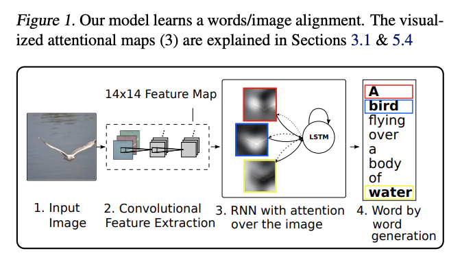
Basic 이미지 캠셔닝은 아래의 방법을 사용한다. Image를 CNN을 통해서 encoder해서 feature를 얻는데 그게 Hidden state h 가 된다. 이 h를 가지고, 맨 위부터 LSTM를 통해서 첫번째 단어와 h1을 얻고, h와 h1을 LSTM에 넣어서 2번째 단어를 얻는다.
나오는 각각의 단어는 이미지의 한 부분만 본다.따라서 이미지 전체를 압축한 h를, 일정 부분만을 보고 결과를 추출해야하는 LSTM에, 넣는 것은 비효율적이다. 이래서 attention mechanism이 필요하다.
attention mechanism 전체 그림
What is an attention model? 위의 이미지에서 Attention Model의 내부는 무엇일까?
attention Model에는 n개의 input이 들어간다. 위의 예시에서 y1 ~ yn이 되겠다.
출력되는 z는 모든 y의 summary 이자, 옆으로 들어가는 c와도 연관된 information이다.
각 변수의 의미
C : context, beginning.
Yi : the representations of the parts of the image. (예를 들어서 이미지 Final feature map의 Channel=n개라면, 1개 Channel을 Yi에 부여한다.)
Z : 다음 단어 예측을 위한 Image filter 값.
attention model 분석하기 (저게 최대 화질 이미지..)
tanh를 통해서 m1,…mn이 만들어 진다. mi는 다른 yj와는 관계없이 생성된다는 것이 중요한 Point이다.
softmax를 사용해서 각 yi를 얼마나 비중있게 봐야 하는가?에 대한 s1,s2…sn값이 나온다. argmax가 hard, softmax를 soft의 개념이라고 한다.
최종 Z는 y1 ,y2 …yn를 s1 ,s2 … sn를 사용해서 the weighted arithmetic mean을 한 것이다.
위 전체 과정을 아래와 같이 수정하는 방법도 있다.
tanh를 dot product로 바꾸기 : any other network, arithmetic(Ex.a dot product) 으로 수정될 수 있다. a dot product 는 두 백터의 연관성을 찾는 것이니, 좀 더 이해하기 쉽다.
hard attention
지금까지 본 것은 “Soft attention (differentiable deterministic mechanism)” 이다. hard attention은 a stochastic process이다. 확률값은 si값을 사용해서 랜덤으로 yi를 선택한다. (the gradient by Monte Carlo sampling)
하지만 gradient 계산이 직관적인 Soft Attention를 대부분 사용한다.
이 이후에, Z를 사용하는LSTM은, i번째 단어를 예측하고 다음에 집중해야하는 영역에 대한 정보를 담은 h_i+1을 return한다.
Learning to Align in Machine Translation (언어 모델에서도 사용해보자)
Image와 다른 점은 attention model에 들어가는 y1,y2 … yi 값은, 문자열이 LSTM을 거쳐나오는 연속적인 hidden layer의 값이라는 것이다.
Attention model을 들여다 보면, 신기하게도 하나의 input당 하나의 output으로 matcing된다. 이것은 translation 과제에서 장점이자, 단점이 될 수 있다.
3. the development of the attention mechanism
핵심 paper
Seq2Seq, or RNN Encoder-Decoder (Cho et al. (2014), Sutskever et al. (2014))
Alignment models (Bahdanau et al. (2015), Luong et al. (2015))
Visual attention (Xu et al. (2015))
Hierarchical attention (Yang et al. (2016))
Transformer (Vaswani et al. (2017))
Sequence to sequence (Seq2Seq) architecture for machine translation
two recurrent neural networks (RNN), namely encoder and decoder.
RNN,LSTM,GRU’s hidden state (from the encoder)를 the decoder에 source information 보낸다.
a fixed-length vector, only last one Hidden state 만을 이용해서 Decoding을 하는 것은 Long sentences issue가 발생할 수 있다.
RNN으로는 Gradient exploding, Gradient vanishing 문제가 크게 일어난다.
multi-head self-attention : 시간 효율적, representation을 하는데 매우 효율적이다. Convolution, recursive operation을 삭제하기 때문이다. 이 모듈에 대해서는 나중에 공부해볼 예정이다.
BERT 는 pretrains bi-directional representations with the improved Transformer architecture. 그리고 XLNet, RoBERTa, GPT-2, and ALBERT 와 같은 논문들이 나오는데에 큰 도움을 주었다.
The famous paper “Attention is all you need” in 2017 changed the way we were thinking about attention
Transformer의 기본 block은 self-attention이다.
Representing the input sentence (sequential 한 데이터를 포현(함축)하는 방법)
transformer 의 탄생 배경 : “entire input sequence를 넣어주는거는 어떨까? 단어 단위로 잘라서 (tokenization) sequential 하게 넣어주지 말고!” (RNN과 LSTM과는 다르다. 그들은 sequentially 하게 일을 처리한다.)
tokenization를 해서 하나의 set을 만든다. 여기에는 단어가 들어가고, 단어간의 order는 중요하지 않다. (irrelevant)
집합 내부 단어들을, (대체, 정사하다) project, (words를) in a distributed geometrical space로, 해야한다. (= word embeddings)
(1) Word Embeddings
character <- word <- sentence와 같이 distributed low-dimensional space로 표현하는 것.
직관적으로 이해해보자. ‘Hello I love you’라는 문장이 있다고 치자. Love는 hello보다는 I와 yout에 더 관련성이 깊을 것이다. 이러한 관련성, 각 단어에 대한 집중 정도를 표현해 주는 것이, 이게 바로 weight를 추가해주는 개념이 되겠다. 아래의 그림은 각 단어와 다른 단어와의 관련성 정도를 나타내주는 확률 표 이다.
I gave my dog Charlie some food. 라는 문장이 있다고 치자. 여기서 gave는 I, dog Charlie, food 모두와 관련 깊은데, 이게 위에서 처럼 weight 개념을 추가해 준다고 바로 해결 될까?? No 아니다. 따라서 우리는 extra attention 개념을 반복해야 한다.
Short residual skip connections
블로그의 필자는, 아래의 Skip Connection구조를 직관적으로 이렇게 설명한다.
인간은 top-down influences (our expectations) 구조를 사용한다. 즉 과거의 기대와 생각이 미래에 본 사물에 대한 판단에 영향을 끼지는 것을 말한다.
Layer Normalization, The linear layer 을 추가적으로 배치해서 Encoder의 성능을 높힌다.
그럼에도 불구하고, domain adaptation을 사용할 수 있는지 없는지 판단하는 방법은, 직접 학습시키고 테스트 해봐야한다.
4. One-Step Domain Adaptation
3가지 basic techniques
divergence-based domain adapatation.
adversarial-based domain adaptation using GAN, domain-confusion loss.
reconstruction using stacked autoencoders.
하나씩 알아가보자.
4-1 Divergence-based Domain Adaptation
some divergence criterion (핵심 차이점 기준?) 을 최소화하고, domain-invariant feature representation 을 찾아내는 것(achieve) (domain 변화에도 변하지 않는 feature extractor Ex. 어떤 신호등 모양이든 같은 신호등feature가 나오도록)
아래에 3가지 방법이 나오는데, 느낌만 가져가기. 뭔 개소리인지 정확히 모르겠다.
(1) MMD - Maximum Mean Discrepancy
two-stream architecture는 파라메터 공유하지 않음.
Soft-max, Regularization(Domain-discrepancy) loss를 사용해서, two-architecture가 similar feature representation(=extractor)가 되도록 만든다.
(2) CORAL - Correlation Alignment
(b)처럼 distribution만 맞춘다고 해서 해결되지 못한다. (c)처럼 soure에 target correlation값을 추가함으로써 align시켜준다.
align the second-order statistics (correlations) instead of the means
label distributions 을 사용한다. (라벨별 확률 분포) by looking at conditional distributions(조건적인 P(확률분포|특정라벨))
두 데이터의 각 라벨에 대해, 교집합 domain feature를 찾는다.
minimizes(최소화 한다) the intra-class discrepancy, maximizing(최대화 한다) the inter-class discrepancy.
좋은논문 : target labels are found by clustering. CCD is minimized.
이런 방법으로
이런 방법을 optimal transport 라고 한다.
두 데이터 간의 feature and label distributions 가 서로 비슷해지게 만들거나,
두 architecture(extractor, representation) 간의 차이가 줄어들게 만든다.
4-2 adversarial-based domain adaptation
source domain에 관련된 인위적인 target data를 만들고, 이 데이터를 사용해서 target network를 학습시킨다. 그리고 진짜 target data를 network에 넣어서 결과를 확인해 본다.
(1) CoGAN - source와 연관성 있는 target data 생성
일부 weight sharing 하는 layer는 domain-invariant feature space extractor로 변해간다.
(2) source/target converter network - source와 연관성 있는 target data 생성
Pixel-Level Domain Transfer (2016 - citation 232)
2개의 discriminator를 사용한다.
첫번째 discriminator는 source에 의해 생성된 target data가 그럴듯 한지 확인하고.
두번째 discriminator는 생성된 target data와 source의 상관성이 있는지 확인한다.
특히 이 방법은 unlabeled data in the target domain 상황에서 사용하기 좋다.
(3) Get rid of generators - 어떤 domain에서도 invariable-feature를 추출하는 extractor 제작
Unsupervised Domain Adaptation by Backpropagation (2015 - citation 2000)
domain confusion loss in addition to the domain classification loss : classificator가 어떤 domain의 data인지 예측하지 못하게 한다.
gradient reversal layer는 the feature distributions를 일치시키기 위해 존재한다.(두 데이터 간의 특징 분포를 일치시키기 위해)
파랑색 부분은 class label를 잘 찾으려고 노력하고
초록색 부분은 domain classifier가 틀리도록 학습되면서(input이미지에 대해서 어떤 domain에서도 invariable-feature를 추출하는 extractor를 만든다), class label을 잘 맞추려고 학습된다.
빨간색은 그대로 domain label을 옳게 classify하도록 학습된다.
Generator & discriminator 구조가 아닌듯, 맞는듯한 신기한 구조를 가지고 있다.
4-3. Reconstruction-based Domain Adaptation
(1) DRCN
Deep Reconstruction-Classification Networks for Unsupervised Domain Adaptation (2016 - citation 435)
(i) classification of the source data (ii) reconstruction of the unlabeled target data
(i) 나중에 input에 target을 넣어도 잘 classifying 하게 만듬. (ii) reconstruction된 data가 task data와 유사하도록 학습된다. 따라서 초반 layer도 task data에 대한 정보를 함축하도록 만들어 진다.
논문에서는, 위 신경망의 Input=Source Reconstruction=Target을 넣고 먼저 학습시킨다. 그리고 반대로 Input=Target Reconstruction=Source가 되도록 다시 학습시켰다고 한다.
아래와 같은 학습 방법도 가능하다.
(2) cycle GANs
(3) conditional GANs
encoder-decoder GAN
conditional GANs are used to translate images from one domain to anothe
Pix2Pix GAN이 대표적이다.
reference를 주면, 그것을 이용해 ouput을 만드는 GAN을 말한다.
5. Conclusion
Deep domain adaptation/ enables us to get closer/ to human-level performance/ in terms of the amount of training data. (원하는 task data (to be relative real-scene)가 적을 때 유용하게 사용할 수 있는 방법이다.)
2. Domain adaptation - Boston Universiry
Domain Adaptation에 대한 설명을 그림으로 아주 재미있게 표현해놓은 좋은 자료.
하지만 아래 내용은 참고만 할 것. 논문을 찾아 읽어봐야 한다.
Applications to different types of domain shift
From dataset to dataset
From simulated to real control
From RGB to depth
From 3D-CAD models to real images
models adapted without labels (NO labels in target domain)
mmdetection/configs : ‘다양한 종류의 신경망’ 모델 설계를 위한, model_config.py 파일이 존재한다.
각 ‘신경망 모델’이름의 폴더에 들어가면, readme.md가 따로 있고, 그곳에 backbone, **style(pytorch/caffe 두가지 framework 사용됨)**, lr-schd, memory, fps, boxAP, cong, Download(model/log) 가 적혀 있어서 참고하면 된다.
생각보다, 거의 Torch, Torchvision 와 같은 큰~모듈 처럼, 내부를 모르는 채로 원하는 함수를 구글링, Official Document 검색으로 찾아서 해야할 만큼 큰 모듈이다. 내가 원하는 모델을 분석하기 위해서 이 패키지를 사용한다는 것은… 멍청한 행동인 것 같다. 그만큼 사소한거 하나하나가 모두 구현되어 있는 큰~모듈이다.
만약 내가 어떤 신경망 모델의 내부 코드가 궁금하다면, Github에서 그 신경망 모델의 이름을 검색하고, 그 신경망만을 위한 코드를 보는것이 낫겠다.
이전에는 이런 생각을 했다. “만약 SSD를 공부하고 싶다면, SSD 패키지를 Github에서 검색해서 사용하는 것 보다는, mmdetection에서 SSD가 어떻게 구현되어 있는지, 어떤 모듈을 사용하는지 찾아보는게 더 좋지 않나? 그게 더 안정화된 코드고 빠른 코드 아닐까? 그래야 내가 혹시 필요한 모듈을 그대로 가져와서 쓸 수 있지 않을까??” 라고 생각했다. 물론 맞는 말이다….
하지만 지금 시간이 급하니.. 정말 필요할 때, ‘2. docs/with existing dataset.md’ 에서 나온 방법을 이용해서, test.py와 train.py를 디버깅하고 어떤 흐름으로, 어떤 함수와 클래스를 이용하며 학습이 되고, 테스트가 되는지 찾아보는 시간을 가지는 것도 좋을 듯 하다.
그럼에도 불구하고, 만약 내가 BlendMask 라는 함수를 수정해서 , 선배님처럼 The Devil Boundary Mask 모델을 만들고 싶다면 mmdetection이나, detectron2를 사용하지 않아도 될 수 있다. 하지만 그래도!! Developer for practice로서, mmdetection과 detectrion2 사용법과 코드가 돌아가는 내부 흐름은 알아두어야 한다고 생각한다.
따라서 개인 컴퓨터가 생기면 디버깅을 하면서, 직접 내부 흐름을 살펴보는 시간도 가져보자.
0. colab 전용 환경 설정
아래에 코드에 간단한, 에러해결의 고민이 적혀있다. 참고해도 좋지만, 새로운 환경에서 mmcv와 mmdetection을 설치하기 위해서, 그냥 주어진 mmcv와 mmdetection의 [github, official_document] 자료를 다시 읽어보고 공부해보는게 더 좋을 듯하다.
fromgoogle.colabimportdrivedrive.mount('/content/drive')%cd/content/drive/MyDrive/GCPcode/torch_package!ls# !pip install torch==1.6.0 torchvision==0.7.0 # -> 오류 발생 이거 때문인지는 모름.
!pipinstall-Utorch==1.5.1+cu101torchvision==0.6.1+cu101-fhttps://download.pytorch.org/whl/torch_stable.htmlimporttorch;torch.__version__# Colab : 아래 나오는 Restart runtime 눌러야 버전 변경 됨.
importtorch;importtorchvisiontorch.__version__,torchvision.__version__# Check nvcc version
!nvcc-V# Check GCC version
!gcc--version# colab error defence
!pipinstalladdict==2.2.1!pipinstallyapf==0.28.0!pipinstallPillow==7.0.0fromaddictimportDictfromyapf.yapflib.yapf_apiimportFormatCode"""
# 이렇게 설치해서 그런지 에러가 나는데..? GCC, GUDA 버전문제라고? torch, GUDA 버전문제라고?
#!git clone https://github.com/open-mmlab/mmcv.git
%cd /content/drive/MyDrive/GCPcode/torch_package/mmcv
!MMCV_WITH_OPS=1 python setup.py develop
# Finished processing dependencies for mmcv-full==1.2.5
# 에러 이름 : linux-gnu.so: undefined symbol
# 해결 : mmcv.__version : 1.2.5 말고 1.2.6으로 설치하게 두니 설치 완료.
# git으로 설치해서 직접 빌드하는 거는 왜... 1.2.5로 다운받아지는 거지? 모르겠다.
"""# mmcv Readmd.md 처럼 위의 셀로, 쿠타, 토치 버전을 알고 mmcv를 정확하게 설치하는 것도 좋은 방법이다.
# pip install mmcv-full -f https://download.openmmlab.com/mmcv/dist/{cu_version}/{torch_version}/index.html
!pipinstallmmcv-full# colab-tuto에는 그냥 이렇게만 설치하니까 나도 일단 이렇게 설치.
# mmcv.__version__ : 1.2.6
importmmcvmmcv.__version__%cd/content/drive/MyDrive/GCPcode/torch_package#!git clone https://github.com/open-mmlab/mmdetection.git
%cd/content/drive/MyDrive/GCPcode/torch_package/mmdetection!pipinstall-rrequirements/build.txt!pipinstall-v-e.# or "python setup.py develop"
importmmdetmmdet.__version__# mmdet 2.8.0
!pythonmmdet/utils/collect_env.py# truble shooting
# Check mmcv installation
frommmcv.opsimportget_compiling_cuda_version,get_compiler_versionprint(get_compiling_cuda_version())print(get_compiler_version())# Check installation
# Check Pytorch installation
importtorch,torchvisionprint(torch.__version__,torch.cuda.is_available())# Check MMDetection installation
importmmdetprint(mmdet.__version__)# Check mmcv installation
frommmcv.opsimportget_compiling_cuda_version,get_compiler_versionprint(get_compiling_cuda_version())print(get_compiler_version())
위에서 확인한 Key를 아래와 같이 수정할 수 있다. . (dot) 을 이용해서 수정이 가능하다.
cfg.dataset_type='KittiTinyDataset'cfg.data_root='kitti_tiny/'cfg.data.test.type='KittiTinyDataset'cfg.data.test.data_root='kitti_tiny/'cfg.data.test.ann_file='train.txt'cfg.data.test.img_prefix='training/image_2'...(mmdetection/demo/MMDet_Tutorial.ipynb파일참조)# The original learning rate (LR) is set for 8-GPU training.
# We divide it by 8 since we only use one GPU.
cfg.optimizer.lr=0.02/8cfg.lr_config.warmup=Nonecfg.log_config.interval=10# Change the evaluation metric since we use customized dataset.
cfg.evaluation.metric='mAP'# We can set the evaluation interval to reduce the evaluation times
cfg.evaluation.interval=12# We can set the checkpoint saving interval to reduce the storage cost
cfg.checkpoint_config.interval=12# print(cfg)를 이쁘게 보는 방법
print(f'Config:\n{cfg.pretty_text}')
여기서 핵심은, cfg.data.test/train/val.type = '내가 아래에 만들 새로운 dataset' 을 집어 넣는 것이다.
Regist Out Dataset
데이터 셋을 다운로드 한후, 우리는 데이터 셋을 COCO format, middle format으로 바꿔줘야 한다.
여기서는 아래이 과정을 수행한다.
from mmdet.datasets.custom import CustomDataset
CustomDataset 을 상속하는 클래스를 만들고 def load_annotations 해주기
아래의 load_annotations에 들어가는 매개변수로, ann_file(type : str)에는 여기서 지정한 파일이 들어간다. cfg.data.test.ann_file = 'train.txt'
train.txt파일의 첫줄을 살펴보면 아래와 같다. Pedestrian 0.00 0 -0.20 712.40 143.00 810.73 307.92 1.89 0.48 1.20 1.84 1.47 8.41 0.01
data_infos는 dict들을 저장해놓은 list이다. In detail, data_infos에는 [ 1장에 이미지에 있는 객체들의 정보를 저장해둔, data_info=dictionary]들이 원소 하나하나로 들어간다.
data_info의 key는 filename, width, height, ann 이다. 특히 ann의 key는 bboxes, labels 등이 있다.
(self.img_prefix 와 같은 CustomDataset 클래스의 맴버변수가 쓰여서 디버깅 못함)
코드 :
importcopyimportos.pathasospimportmmcvimportnumpyasnpfrommmdet.datasets.builderimportDATASETSfrommmdet.datasets.customimportCustomDataset@DATASETS.register_module()classKittiTinyDataset(CustomDataset):CLASSES=('Car','Pedestrian','Cyclist')defload_annotations(self,ann_file):cat2label={k:ifori,kinenumerate(self.CLASSES)}# load image list from file
image_list=mmcv.list_from_file(self.ann_file)data_infos=[]# convert annotations to middle format
forimage_idinimage_list:filename=f'{self.img_prefix}/{image_id}.jpeg'image=mmcv.imread(filename)height,width=image.shape[:2]data_info=dict(filename=f'{image_id}.jpeg',width=width,height=height)# load annotations
label_prefix=self.img_prefix.replace('image_2','label_2')lines=mmcv.list_from_file(osp.join(label_prefix,f'{image_id}.txt'))content=[line.strip().split(' ')forlineinlines]bbox_names=[x[0]forxincontent]bboxes=[[float(info)forinfoinx[4:8]]forxincontent]# 진짜 필요한 변수
gt_bboxes=[]gt_labels=[]# 사용하지 않은 변수
gt_bboxes_ignore=[]gt_labels_ignore=[]# filter 'DontCare'
forbbox_name,bboxinzip(bbox_names,bboxes):ifbbox_nameincat2label:gt_labels.append(cat2label[bbox_name])gt_bboxes.append(bbox)else:gt_labels_ignore.append(-1)gt_bboxes_ignore.append(bbox)data_anno=dict(bboxes=np.array(gt_bboxes,dtype=np.float32).reshape(-1,4),labels=np.array(gt_labels,dtype=np.long),bboxes_ignore=np.array(gt_bboxes_ignore,dtype=np.float32).reshape(-1,4),labels_ignore=np.array(gt_labels_ignore,dtype=np.long))data_info.update(ann=data_anno)data_infos.append(data_info)returndata_infos
coco_json_file 에 image의 path와 image의 annotation정보가 모두 있기 때문에, 사실 우리의 python 코드는 json 하나만 보면 된다!!
따라서 CSV이든 XML이든 어떤 파일 형식으로 annotation된 데이터가 있다면, coco 즉 json포멧으로 annotation을 바꾸는 코드가 분명 있을거야. github에도 있을거고, 나의 블로그 Post에 【Tensorflow】, 【Keras】파일에도 이에 대한 내용이 잇었으니까 참고하도록 하자.
mmdetection에서도 mmcv를 이용해서 어떤 파일형식이든, coco format형식으로 바꿔주는, def convert_balloon_to_coco(ann_file, out_file, image_prefix): 함수를 예시로 주어주었다. 가능하다면 이것을 사용해도 좋은 듯 하다.
(2) Prepare a config
ballon dataset을 사용하기 위해, 어떻게 mask_rcnn_r50_caffe_fpn_mstrain-poly_1x_balloon.py 파일을 만들었는지 나와 있으니 참고하도록 하자. (config.py 링크)
위의 KittiTiny는 from mmdet.datasets.custom import CustomDataset 를 상속받아서 dataset을 만들어서 그런지, the number of class에 대한 고려는 안했지만, 여기서는 json파일을 직접 만들었기 때문에 #class를 고려를 해줬다.
(3) Train, test, inference models on the customized dataset.
더 다양한 case에 대한 agupare 적용방법은, 2. docs/with existing dataset.md 파일 참조
4. webcam_demo.py
model=init_detector(args.config,args.checkpoint,device=device)camera=cv2.VideoCapture(args.camera_id)print('Press "Esc", "q" or "Q" to exit.')whileTrue:ret_val,img=camera.read()result=inference_detector(model,img)ch=cv2.waitKey(1)ifch==27orch==ord('q')orch==ord('Q'):breakmodel.show_result(img,result,score_thr=args.score_thr,wait_time=1,show=True)
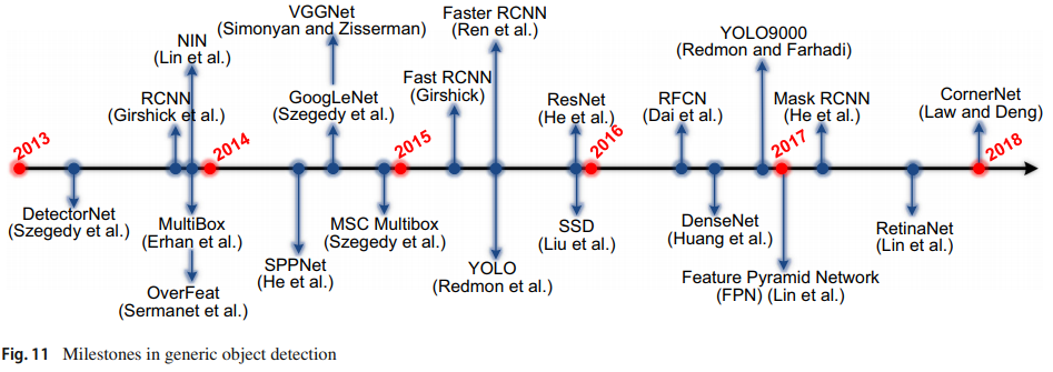
20, 200, 91 object classes / VOC, ILSVRC, COCO is much smaller than can be recognized by humans.
Efficiency and Scalability Related Challenges
mobile/wearable devices have limited computational capabilities and storage space
A further challenge is that of scalability : unseen objects, unknown situations, it may become impossible to annotate them manually, forcing a reliance on weakly supervised strategies.
2.3 Progress in the Past 2 Decades
accurate annotations are labor intensive to obtain
Ability to detect many object categories matches that of humans(인간 같은) 3000~3000 categories is undoubtedly an unresolved problem so far.
3. A Brief Introduction to Deep Learning
pass
4.1 Dataset
PASCAL VOC
ImageNet
MS COCO
Places
Open Images
4.2 Evaluation Criteria
Frames Per Second (FPS)
precision, and recall.
Average Precision (AP) -> over all object categories, the mean AP (mAP)
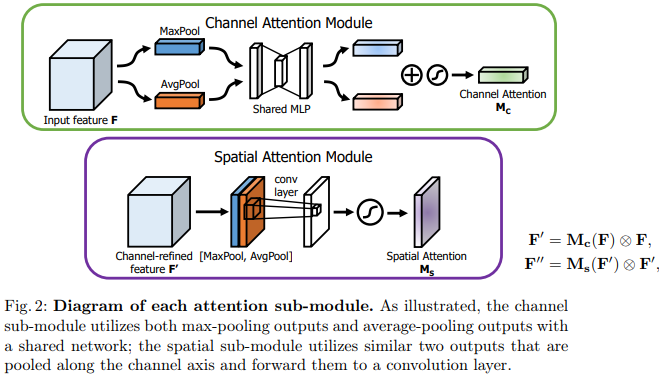
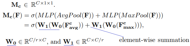
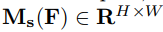
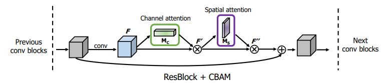
our module sequentially infers attention maps along two separate dimensions
the attention maps are multiplied to the input feature map for adaptive feature refinement (향상되어 정제된 feature)
lightweight and general module, it can be integrated into any CNN architectures
1. introduction
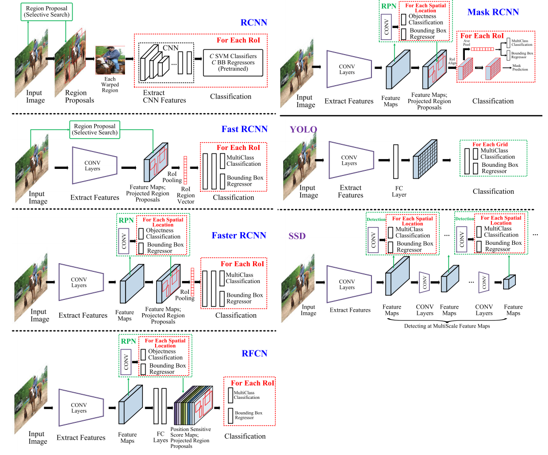
Recent Detectors
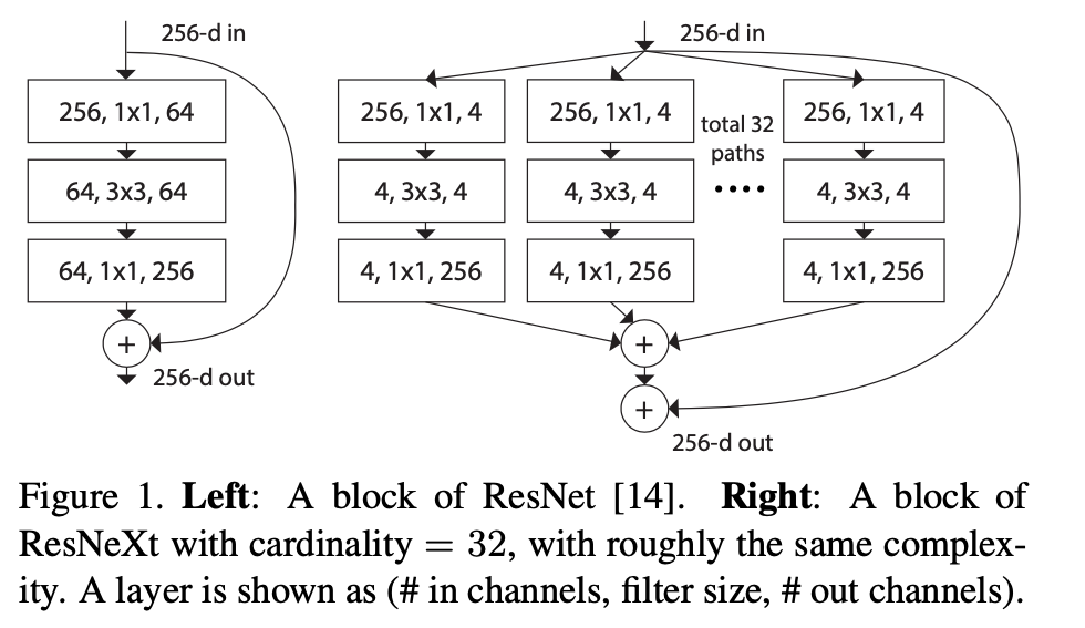
recent researches have mainly investigated depth, width(#channel), and cardinality(같은 형태의 빌딩 블록의 갯수).
VGGNet, ResNet, GoogLeNet has become deeper for rich representation(중요한 특징 표현력).
GoogLeNet and Wide ResNet(2016), width must be another important factor.
Xception and ResNeXt, increase the cardinality of a network . the cardinality saves the total number of parameters and make results powerful than depth and width.
significant visual attention papers
[16] A recurrent neural network for image generation
[17] Spatial transformer networks
Emphasize meaningful features / along those two principal dimensions / channel(depth) and spatial axes(x,y). -> channel and spatial attention modules -> learning which information to emphasize or suppress.
Contribution
Can be widely applied to boost representation power of CNNs
따라서 목차를 보고 ‘이런 내용이 있구나’하고 나중에 필요하면, 와서 듣자. 지금은 진짜 궁금한것만 듣자.
OpenCV-Python 시작하기
Ch 01. OpenCV-Python 시작하기 - 01. 전체 코스와 컴퓨터 비전 소개
Ch 01. OpenCV-Python 시작하기 - 02. 영상의 구조와 표현
Ch 01. OpenCV-Python 시작하기 - 03. OpenCV 소개와 설치
Ch 01. OpenCV-Python 시작하기 - 04. VS Code 설치와 개발 환경 설정
Ch 01. OpenCV-Python 시작하기 - 05. 영상 파일 불러와서 출력하기
Ch 01. OpenCV-Python 시작하기 - 06. OpenCV 주요 함수 설명
Ch 01. OpenCV-Python 시작하기 - 07. Matplotlib 사용하여 영상 출력하기
Ch 01. OpenCV-Python 시작하기 - 08. 실전 코딩 - 이미지 슬라이드쇼
OpenCV-Python 기초 사용법
Ch 02. OpenCV-Python 기초 사용법 - 01. 영상의 속성과 픽셀 값 처리
Ch 02. OpenCV-Python 기초 사용법 - 02. 영상의 생성, 복사, 부분 영상 추출
Ch 02. OpenCV-Python 기초 사용법 - 03. 마스크 연산과 ROI
Ch 02. OpenCV-Python 기초 사용법 - 04. OpenCV 그리기 함수
Ch 02. OpenCV-Python 기초 사용법 - 05. 카메라와 동영상 처리하기 1
Ch 02. OpenCV-Python 기초 사용법 - 06. 카메라와 동영상 처리하기 2
Ch 02. OpenCV-Python 기초 사용법 - 07. 키보드 이벤트 처리하기
Ch 02. OpenCV-Python 기초 사용법 - 08. 마우스 이벤트 처리하기
Ch 02. OpenCV-Python 기초 사용법 - 09. 트랙바 사용하기
Ch 02. OpenCV-Python 기초 사용법 - 10. 연산 시간 측정 방법
Ch 02. OpenCV-Python 기초 사용법 - 11. 실전 코딩 - 동영상 전환 이펙트
기본적인 영상 처리 기법
Ch 03. 기본적인 영상 처리 기법 - 01. 영상의 밝기 조절
Ch 03. 기본적인 영상 처리 기법 - 02. 영상의 산술 및 논리 연산
Ch 03. 기본적인 영상 처리 기법 - 03. 컬러 영상 처리와 색 공간
Ch 03. 기본적인 영상 처리 기법 - 04. 히스토그램 분석
Ch 03. 기본적인 영상 처리 기법 - 05. 영상의 명암비 조절
Ch 03. 기본적인 영상 처리 기법 - 06. 히스토그램 평활화
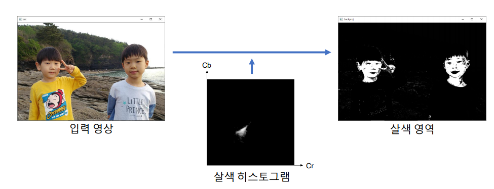
Ch 03. 기본적인 영상 처리 기법 - 07. 특정 색상 영역 추출하기
Ch 03. 기본적인 영상 처리 기법 - 08. 히스토그램 역투영
Ch 03. 기본적인 영상 처리 기법 - 09. 실전 코딩 - 크로마키 합성
필터링
Ch 04. 필터링 - 01. 필터링 이해하기
Ch 04. 필터링 - 02. 블러링 (1) - 평균값 필터
Ch 04. 필터링 - 03. 블러링 (2) - 가우시안 필터
Ch 04. 필터링 - 04. 샤프닝 - 언샤프 마스크 필터
Ch 04. 필터링 - 05. 잡음 제거 (1) - 미디언 필터
Ch 04. 필터링 - 06. 잡음 제거 (2) - 양방향 필터
Ch 04. 필터링 - 07. 실전 코딩 - 카툰 필터 카메라
기하학적 변환
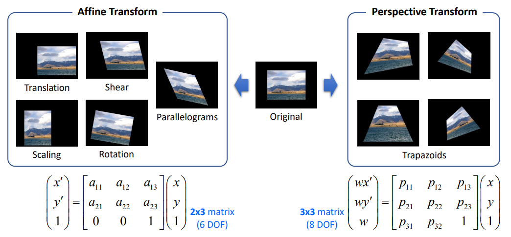
Ch 05. 기하학적 변환 - 01. 영상의 이동 변환과 전단 변환
Ch 05. 기하학적 변환 - 02. 영상의 확대와 축소
Ch 05. 기하학적 변환 - 03. 이미지 피라미드
Ch 05. 기하학적 변환 - 04. 영상의 회전
Ch 05. 기하학적 변환 - 05. 어파인 변환과 투시 변환
Ch 05. 기하학적 변환 - 06. 리매핑
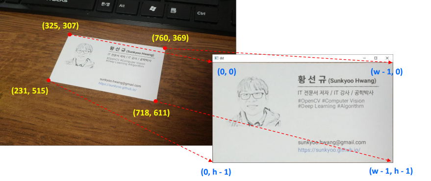
Ch 05. 기하학적 변환 - 07. 실전 코딩 - 문서 스캐너
영상의 특징 추출
CH 06. 영상의 특징 추출 - 01. 영상의 미분과 소베 필터
CH 06. 영상의 특징 추출 - 02. 그래디언트와 에지 검출
CH 06. 영상의 특징 추출 - 03. 캐니 에지 검출
CH 06. 영상의 특징 추출 - 04. 허프 변환 직선 검출
CH 06. 영상의 특징 추출 - 05. 허프 원 변환 원 검출
CH 06. 영상의 특징 추출 - 06. 실전 코딩 동전 카운터
이진 영상 처리
CH 07. 이진 영상 처리 - 01. 영상의 이진화
CH 07. 이진 영상 처리 - 02. 자동 이진화 Otsu 방법
CH 07. 이진 영상 처리 - 03. 지역 이진화
CH 07. 이진 영상 처리 - 04. 모폴로지 (1) 침식과 팽창
CH 07. 이진 영상 처리 - 05. 모폴로지 (2) 열기와 닫기
CH 07. 이진 영상 처리 - 06. 레이블링
CH 07. 이진 영상 처리 - 07. 외곽선 검출
CH 07. 이진 영상 처리 - 08. 다양한 외곽선 함수
CH 07. 이진 영상 처리 - 09. 실전 코딩 명함 인식 프로그램
영상 분할과 객체 검출
CH 08. 영상 분할과 객체 검출 - 01. 그랩컷
CH 08. 영상 분할과 객체 검출 - 02. 모멘트 기반 객체 검출
CH 08. 영상 분할과 객체 검출 - 03. 템플릿 매칭 (1) 이해하기
CH 08. 영상 분할과 객체 검출 - 04. 템플릿 매칭 (2) 인쇄체 숫자 인식
CH 08. 영상 분할과 객체 검출 - 05. 캐스케이드 분류기 - 얼굴 검출
CH 08. 영상 분할과 객체 검출 - 06. HOG 보행자 검출
CH 08. 영상 분할과 객체 검출 - 07. 실전 코딩 간단 스노우 앱
특징점 검출과 매칭
CH 09. 특징점 검출과 매칭 - 01. 코너 검출
CH 09. 특징점 검출과 매칭 - 02. 특징점 검출
CH 09. 특징점 검출과 매칭 - 03. 특징점 기술
CH 09. 특징점 검출과 매칭 - 04. 특징점 매칭
CH 09. 특징점 검출과 매칭 - 05. 좋은 매칭 선별
CH 09. 특징점 검출과 매칭 - 06. 호모그래피와 영상 매칭
CH 09. 특징점 검출과 매칭 - 07. 이미지 스티칭
CH 09. 특징점 검출과 매칭 - 08. 실전 코딩 - AR 비디오 플레이어
객체 추적과 모션 벡터
CH 10. 객체 추적과 모션 벡터 - 01. 배경 차분 정적 배경 차분
CH 10. 객체 추적과 모션 벡터 - 02. 배경 차분 이동 평균 배경
CH 10. 객체 추적과 모션 벡터 - 03. 배경 차분 MOG 배경 모델
CH 10. 객체 추적과 모션 벡터 - 04. 평균 이동 알고리즘
CH 10. 객체 추적과 모션 벡터 - 05. 캠시프트 알고리즘
CH 10. 객체 추적과 모션 벡터 - 06. 루카스 - 카나데 옵티컬플로우
CH 10. 객체 추적과 모션 벡터 - 07. 밀집 옵티컬플로우
CH 10. 객체 추적과 모션 벡터 - 08. OpenCV 트래커
CH 10. 객체 추적과 모션 벡터 - 09. 실전 코딩 - 핸드 모션 리모컨
머신러닝
CH 11. 머신 러닝 - 01. 머신 러닝 이해하기
CH 11. 머신 러닝 - 02. OpenCV 머신 러닝 클래스
CH 11. 머신 러닝 - 03. k최근접 이웃 알고리즘
CH 11. 머신 러닝 - 04. KNN 필기체 숫자 인식
CH 11. 머신러닝 - 05. SVM 알고리즘
CH 11. 머신러닝 - 06. OpenCV SVM 사용하기
CH 11. 머신러닝 - 07. HOG SVM 필기체 숫자 인식
CH 11. 머신러닝 - 08. 숫자 영상 정규화
CH 11. 머신러닝 - 09. k-평균 알고리즘
CH 11. 머신러닝 - 10. 실전 코딩 문서 필기체 숫자 인식
딥러닝 이해와 영상 인식
CH 12. 딥러닝 이해와 영상 인식 - 01. 딥러닝 이해하기
CH 12. 딥러닝 이해와 영상 인식 - 02. CNN 이해하기
CH 12. 딥러닝 이해와 영상 인식 - 03. 딥러닝 학습과 모델 파일 저장
CH 12. 딥러닝 이해와 영상 인식 - 04. OpenCV DNN 모듈
CH 12. 딥러닝 이해와 영상 인식 - 05. MNIST 학습 모델 사용하기
CH 12. 딥러닝 이해와 영상 인식 - 06. GoogLeNet 영상 인식
CH 12. 딥러닝 이해와 영상 인식 - 07. 실전 코딩 한글 손글씨 인식
딥러닝 활용 : 객체 검출, 포즈 인식
CH 13. 딥러닝 활용 객체 검출 - 01. OpenCV DNN 얼굴 검출
CH 13. 딥러닝 활용 객체 검출 - 02. YOLOv3 객체 검출
CH 13. 딥러닝 활용 객체 검출 - 03. Mask-RCNN 영역 분할
CH 13. 딥러닝 활용 객체 검출 - 04. OpenPose 포즈 인식
CH 13. 딥러닝 활용 객체 검출 - 05. EAST 문자 영역 검출
CH 13. 딥러닝 활용 객체 검출 - 06. 실전 코딩 얼굴 인식
importsysimportcv2print(cv2.__version__)img=cv2.imread('cat.bmp')ifimgisNone:print('Image load failed!')sys.exit()cv2.namedWindow('image')cv2.imshow('image',img)cv2.waitKey()# 아무키나 누르면 window 종료
cv2.destroyAllWindows()
importmatplotlib.pyplotaspltimportcv2# 컬러 영상 출력
imgBGR=cv2.imread('cat.bmp')imgRGB=cv2.cvtColor(imgBGR,cv2.COLOR_BGR2RGB)# cv2.IMREAD_GRAYSCALE
plt.axis('off')plt.imshow(imgRGB)# cmap='gray'
plt.show()# subplot
plt.subplot(121),plt.axis('off'),plt.imshow(imgRGB)plt.subplot(122),plt.axis('off'),plt.imshow(imgGray,cmap='gray')plt.show()
8강 - 이미지 슬라이드쇼 프로그램
폴더에서 파일 list 가져오기
importosfile_list=os.listdir('.\\images')img_files=[fileforfileinfile_listiffile.endswith('.jpg')]# 혹은
importglobimg_files=glob.glob('.\\images\\*.jpg')
전체 화면 영상 출력
cv2.namedWindow('image',cv2.WINDOW_NORMAL)# normal 이여야 window 창 변경 가능.
cv2.setWindowProperty('image',cv2.WND_PROP_FULLSCREEN,cv2.WINDOW_FULLSCREEN)
반복적으로, 이미지 출력
cnt=len(img_files)idx=0whileTrue:img=cv2.imread(img_files[idx])ifimgisNone:print('Image load failed!')breakcv2.imshow('image',img)ifcv2.waitKey(1000)>=27:# 1초 지나면 False, ESC누루면 True
break# while 종료
# cv2.waitKey(1000) -> 1
# cv2.waitKey(1000) >= 0: 아무키나 누르면 0 초과의 수 return
idx+=1ifidx>=cnt:idx=0
img3 = img1.copy() -> 새로운 메모리에 이미지 정보 다시 할당 array안의 array도 다시 할당한다. 여기서는 deepcopy랑 같다. ](https://junha1125.github.io/docker-git-pytorch/2021-01-07-torch_module_research/#21-copydeepcopy)
numpy에서는 deepcopy랑 copy가 같다. 라고 외우자
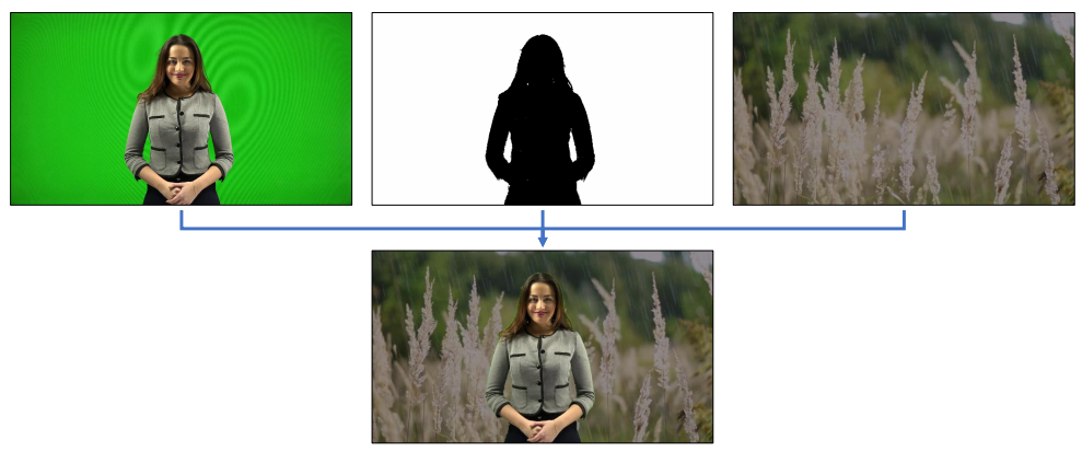
2-3강 - 마스크 연산과 ROI
마스크 영상으로는 0 또는 255로 구성된 이진 영상(binary image), Gray Scale
cv2.copyTo(src, mask, dst=None) -> dst
src=cv2.imread('airplane.bmp',cv2.IMREAD_COLOR)mask=cv2.imread('mask_plane.bmp',cv2.IMREAD_GRAYSCALE)dst=cv2.imread('field.bmp',cv2.IMREAD_COLOR)cv2.copyTo(src,mask,dst1)dst2=cv2.copyTo(src,mask)# 하지만 아래와 같은 슬라이딩 연산도 가능!!
dst[mask>0]=src[mask>0]# -> dist = dst1
src, mask, dst는 w,h 모두 크기가 같아야 함. src와 dst는 같은 타입. mask는 그레이스케일 타입의 이진 영상.
dst2 :
dst과 dst2는 완전히 다른 이미지로 생성되니 주의해서 사용할 것.
투명한 배경이 있는 png 파일 (4channel)
src=cv2.imread('airplane.bmp',cv2.IMREAD_UNCHANGED)## 투명배경 있는 것은 IMREAD_UNCHANGED!!!
mask=src[:,:,-1]src=src[;,:,0:3]h,w=src.shape[:2]crop=dst[x:x+h,y:w+2]# src, mask, dst는 w,h 모두 크기가 같아야 함
cv2.copyTo(src,mask,crop)
2-4강 - OpenCV그리기 함수
주의할 점 : in-place 알고리즘 -> 원본 데이터 회손
자세한 내용은 인강 참조, 혹은 OpenCV 공식 문서 참조 할 것.
직선 그리기 : cv2.line
사각형 그리기 : cv2.rectangle
원 그리기 : cv2.circle
다각형 그리기 : cv2.polylines
문자열 출력 : cv2.putText
5강 - 카메라와 동영상 처리하기 1
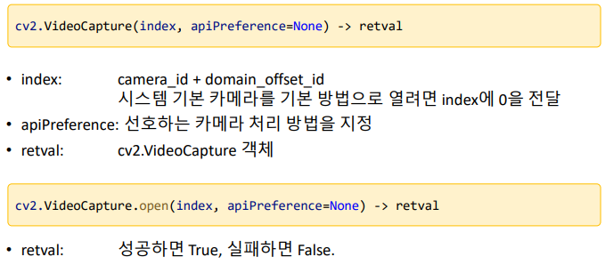
OpenCV에서는 카메라와 동영상으로부터 프레임(frame)을 받아오는 작업을 cv2.VideoCapture 클래스 하나로 처리함
카메라 열기
index : 2대가 있으면 테스트 해봐서 0,1번 중 하나 이다. domain_offset_id는 무시하기(카메라를 Open하는 방법을 운영체제가 적절한 방법을 사용한다.)
importsysimportcvcap=cv2.VideoCapture()cap.open(0)# 혹은 위의 2줄 한줄로 cap = cv2.VideoCapture(0)
ifnotcap.isOpend()print('camera open failed!')sys.exit()whileTure:ret,frame=cap.read()ifnotret:# frame을 잘 받아 왔는가? # 가장 마지막 프레임에서 멈춘다
breakedge=cv2.Canny(frame,50,150)cv2.imshow('edge',edge)# 2개의 창이 뜬다!! figure 설정할 필요 없음
cv2.imshow('frame',frame)cv2.waitKey(20)==27:# ESC눌렀을떄
breakcap.release()# cap 객체 delete
cv2.destroyAllWindows()
동영상 열기
위의 코드에서 cap = cv2.VideoCapture(‘Video File Path’) 를 넣어주고 나머지는 위에랑 똑같이 사용하면 된다.
이미지 반전 : inversed = ~frame. RGB 중 Grean = 0, RB는 255에 가까워짐
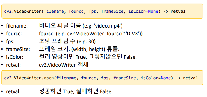
# 나의 카메로 open
cap=cv2.VideoCapture(0)w=round(cap.get(cv2.CAP_PROP_FRAME_WIDTH))h=round(cap.get(cv2.CAP_PROP_FRAME_HEIGHT))# 동영상 준비 중
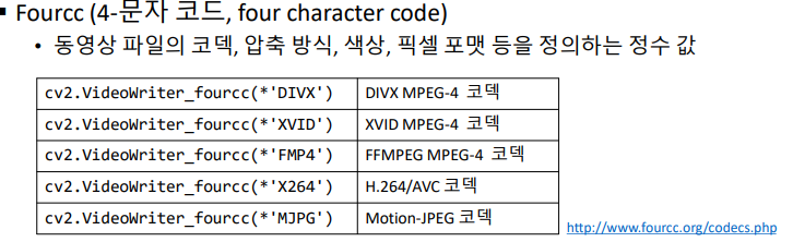
fourcc=cv2.VideoWriter_fourcc(*'DIVX')# *'DIVX' == 'D','I','V','X'
fps=30delay=round(1000/fps)# 프레임과 프레임 사이의 시간간격 (1000ms/30fps)
out=cv2.VideoWriter('output.avi',fourcc,30,(w,h))ifnotout.isOpened():print('File open failed!')cap.release()sys.exit()whileTrue:ret,frame=cap.read()ifnotret:breakinversed=~frame# 반전하는 코드. RGB 중 Grean = 0, RB는 255에 가까워짐
# 신기하니, 아래의 cv2.imshow('inversed', inversed) 결과 확인해보기.
"""
edge = cv2.Canny(frame,50,150)
edge_color = cv2.cvtColor(edge,cv2.COLOR_GRAY2BGR)
out.write(edge_color)
"""out.write(frame)cv2.imshow('frame',frame)cv2.imshow('inversed',inversed)ifcv2.waitKey(delay)==27:# delay는 이와 같이 사용해도 좋다. 없어도 됨.
break
2-7장 - 키보드 이벤트 처리하기
cv2.waitKey(delay=None) -> retval
while True: 문을 계속 돌면서, 매 시간 마다 키보드 input이 없으면 필요없는 값을 return하고 while문에는 영향을 끼치지 않는다.
# 키보드에서 'i' 또는 'I' 키를 누르면 영상을 반전
importcv2img=cv2.imread('cat.bmp',cv2.IMREAD_GRAYSCALE)cv2.imshow('image',img)whileTrue:keycode=cv2.waitKey()ifkeycode==ord('i')orkeycode==ord('I'):img=~imgcv2.imshow('image',img)elifkeycode==27:breakcv2.destroyAllWindows()
2-8장 - 마우스 이벤트 처리하기
마우스 이벤트 콜백함수 등록 함수 : cv2.setMouseCallback(windowName, onMouse, param=None) -> None
마우스 이벤트 처리 함수(콜백 함수) 형식 : onMouse(event, x, y, flags, param) -> None
# 두 개의 동영상을 열어서 cap1, cap2로 지정
cap1=cv2.VideoCapture('video1.mp4')cap2=cv2.VideoCapture('video2.mp4')ifnotcap1.isOpened()ornotcap2.isOpened():print('video open failed!')sys.exit()# 두 동영상의 크기, FPS는 같다고 가정함
frame_cnt1=round(cap1.get(cv2.CAP_PROP_FRAME_COUNT))# 15초 * 24 = Total 360 frame
frame_cnt2=round(cap2.get(cv2.CAP_PROP_FRAME_COUNT))fps=cap1.get(cv2.CAP_PROP_FPS)# 24
effect_frames=int(fps*2)# 48 -> 1번 동영상의 맨 뒤 48프레임과, 2번 동영상의 맨 앞 48프레임이 겹친다
print('frame_cnt1:',frame_cnt1)print('frame_cnt2:',frame_cnt2)print('FPS:',fps)delay=int(1000/fps)w=round(cap1.get(cv2.CAP_PROP_FRAME_WIDTH))h=round(cap1.get(cv2.CAP_PROP_FRAME_HEIGHT))fourcc=cv2.VideoWriter_fourcc(*'DIVX')# 출력 동영상 객체 생성
out=cv2.VideoWriter('output.avi',fourcc,fps,(w,h))# 1번 동영상 복사
foriinrange(frame_cnt1-effect_frames):ret1,frame1=cap1.read()ifnotret1:print('frame read error!')sys.exit()out.write(frame1)print('.',end='')cv2.imshow('output',frame1)cv2.waitKey(delay)# 1번 동영상 뒷부분과 2번 동영상 앞부분을 합성
foriinrange(effect_frames):ret1,frame1=cap1.read()ret2,frame2=cap2.read()ifnotret1ornotret2:print('frame read error!')sys.exit()dx=int(w/effect_frames)*iframe=np.zeros((h,w,3),dtype=np.uint8)frame[:,0:dx,:]=frame2[:,0:dx,:]frame[:,dx:w,:]=frame1[:,dx:w,:]#alpha = i / effect_frames
#frame = cv2.addWeighted(frame1, 1 - alpha, frame2, alpha, 0)
out.write(frame)print('.',end='')cv2.imshow('output',frame)cv2.waitKey(delay)# 2번 동영상을 복사
foriinrange(effect_frames,frame_cnt2):ret2,frame2=cap2.read()ifnotret2:print('frame read error!')sys.exit()out.write(frame2)print('.',end='')cv2.imshow('output',frame2)cv2.waitKey(delay)print('\noutput.avi file is successfully generated!')cap1.release()cap2.release()out.release()cv2.destroyAllWindows()```
chap3 - 기본 영상 처리 기법
Ch 03. 기본적인 영상 처리 기법 - 01. 영상의 밝기 조절
밝기 조절을 위한 함수 : cv2.add(src1, src2, dst=None, mask=None, dtype=None) -> dst
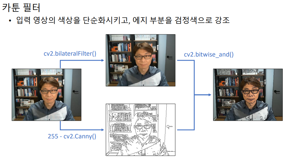
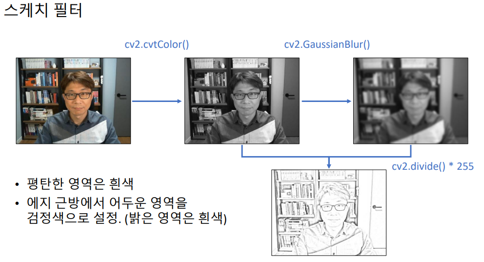
# 카툰 필터 카메라
importsysimportnumpyasnpimportcv2defcartoon_filter(img):h,w=img.shape[:2]img2=cv2.resize(img,(w//2,h//2))blr=cv2.bilateralFilter(img2,-1,20,7)edge=255-cv2.Canny(img2,80,120)edge=cv2.cvtColor(edge,cv2.COLOR_GRAY2BGR)dst=cv2.bitwise_and(blr,edge)# 논리 연산자
dst=cv2.resize(dst,(w,h),interpolation=cv2.INTER_NEAREST)returndstdefpencil_sketch(img):gray=cv2.cvtColor(img,cv2.COLOR_BGR2GRAY)blr=cv2.GaussianBlur(gray,(0,0),3)dst=cv2.divide(gray,blr,scale=255)returndstcap=cv2.VideoCapture(0)ifnotcap.isOpened():print('video open failed!')sys.exit()cam_mode=0whileTrue:ret,frame=cap.read()ifnotret:breakifcam_mode==1:frame=cartoon_filter(frame)elifcam_mode==2:frame=pencil_sketch(frame)frame=cv2.cvtColor(frame,cv2.COLOR_GRAY2BGR)cv2.imshow('frame',frame)key=cv2.waitKey(1)ifkey==27:breakelifkey==ord(' '):cam_mode+=1ifcam_mode==3:cam_mode=0cap.release()cv2.destroyAllWindows()
chap5 - 기하학적 변환
수학적 공식은 ‘20년2학기/윤성민 교수님 컴퓨터 비전 수업 자료 참조’
cv2.warpAffine(src, M, dsize, dst=None, flags=None, borderMode=None, borderValue=None) -> dst
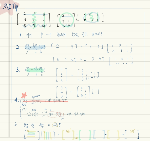
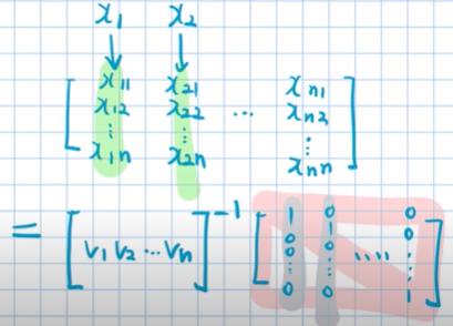
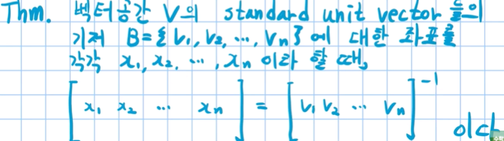
E = {e1,e2,e3 … en} -> V = {v1,v2,v3 … vn} | e1과 v1은 백터 | v끼리는 서로 정규일 필요는 없다.
아래에서 x(kn) 은 V의 원소들의 선형결합 계수 이다.
xk1v1 * xk2v2 * xk3v3 * … xknvn = ek | k = 1~n까지 n차 연립방정식
위의 n개의 연립방정식으로 행렬로 표현하면 아래와 같다.
정리 :
일반화 (48강에서 증명)
(x1,x2 … xn)B = B의 기저백터들에 x1,x2,x3..xn의 계수로의 선형결합
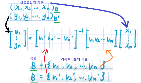
예시
해석 : B를 기저로 하는 좌표값이 x1~xn 이라면, 그 좌표를 B’을 기저로하는 좌표값으로 바꾸면 어떤 좌표 y1~yn이 되는가? 에 대한 공식이다.
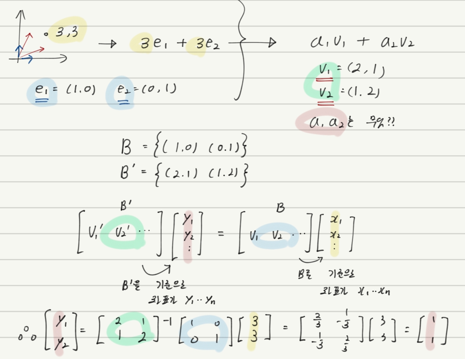
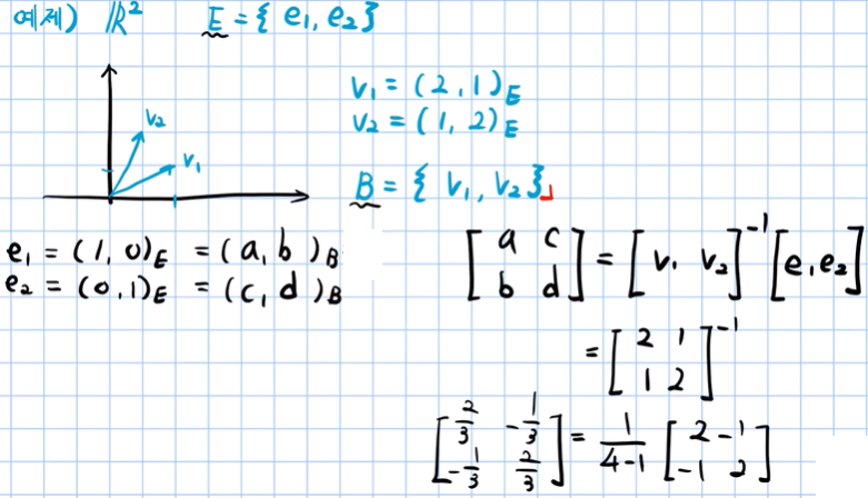
예제 :
(2,1)E는 E의 백터들에 2와 1의 계수로 선형결합 해준 백터 = v1 을 의미함.
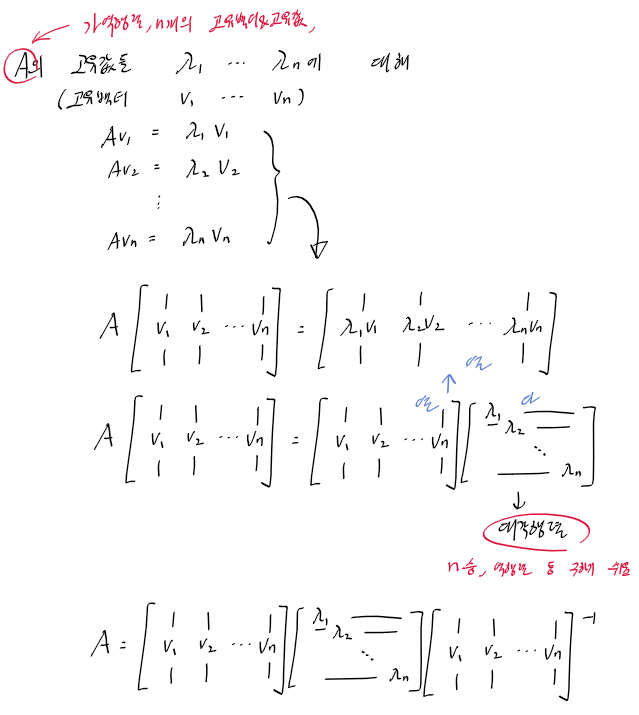
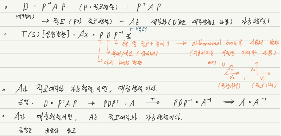
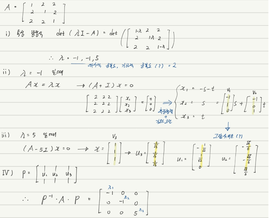
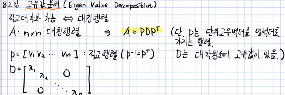
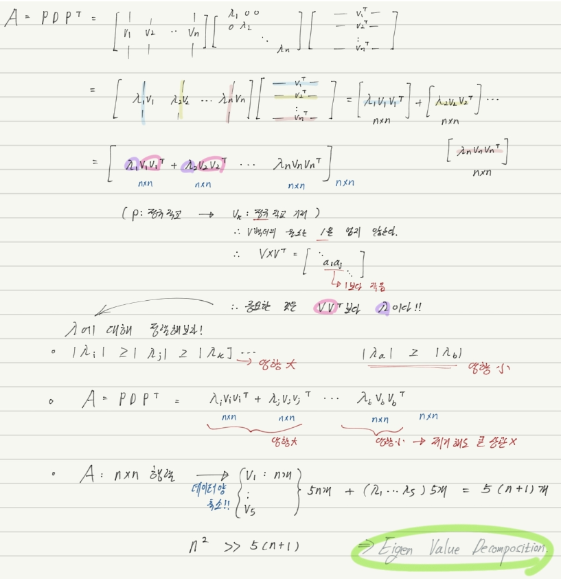
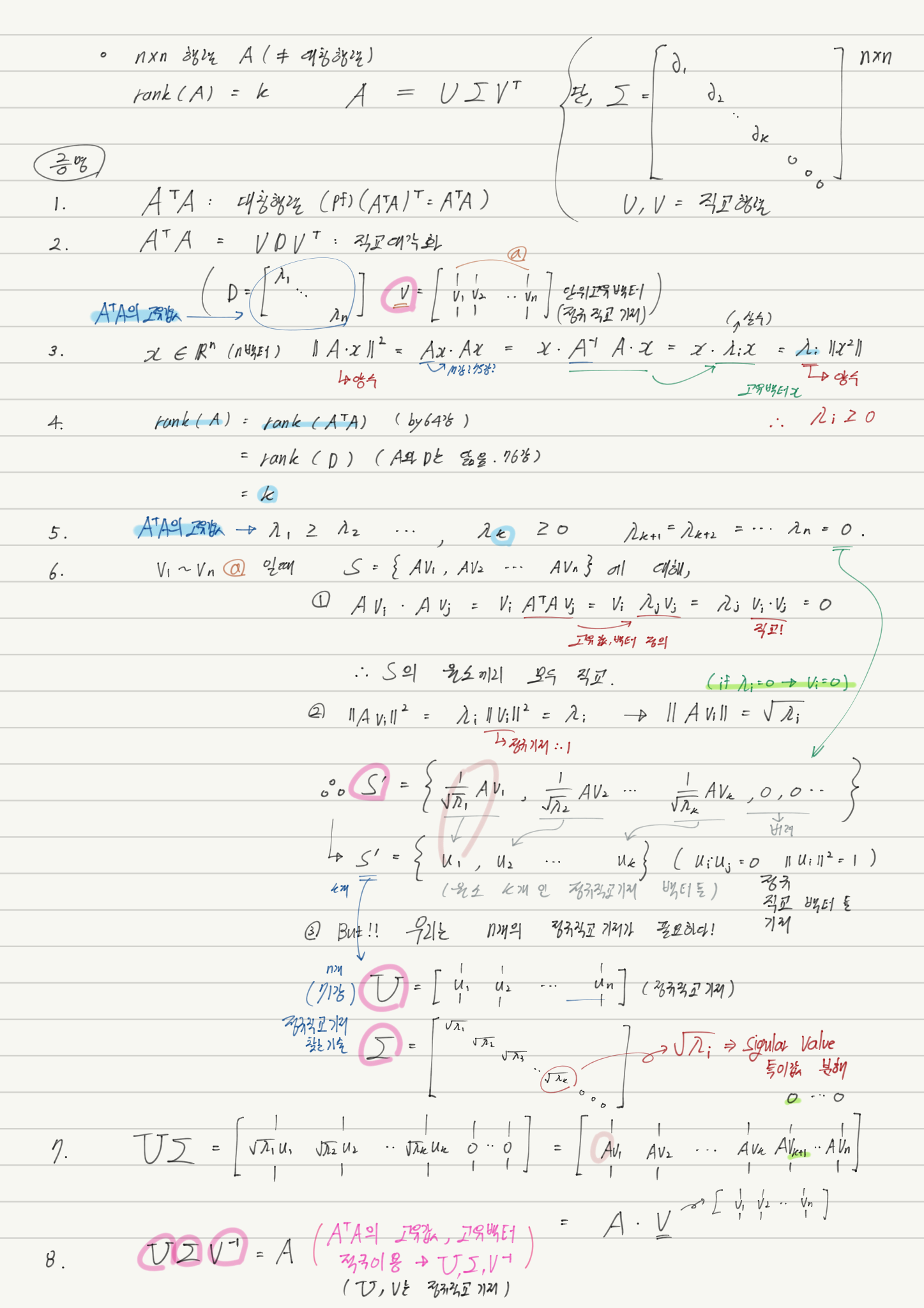
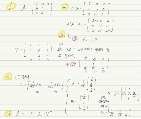
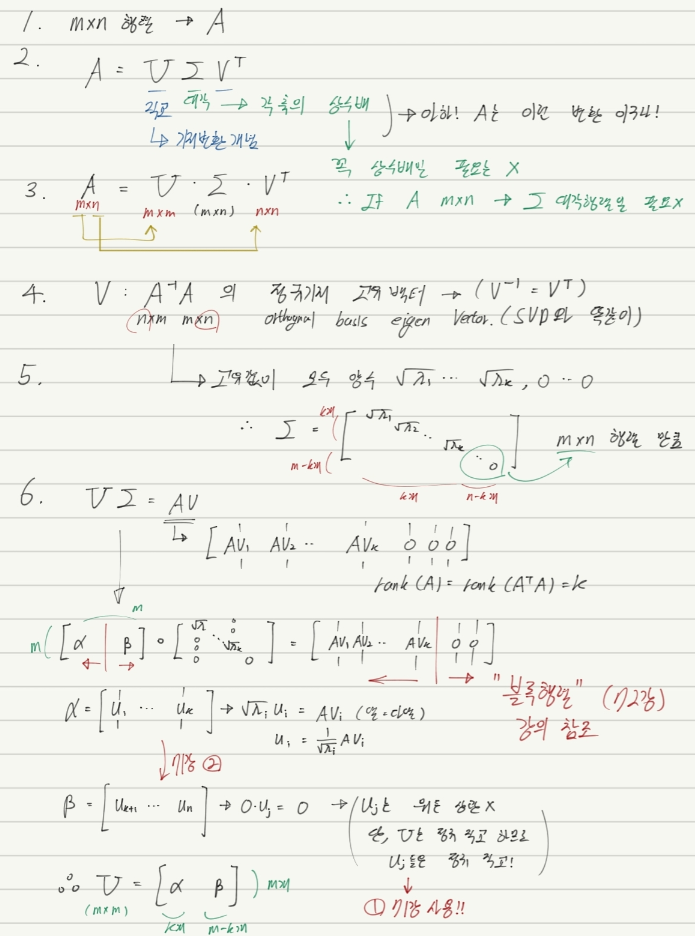
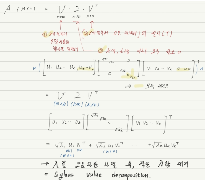
48강 기저변환과 대각화(= EVD(Eigen Value Decomposition) 기초)
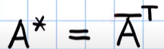
대각화 : P * A * inverse(P) = D’(대각행렬) -> A =inverse(P) * D’(대각행렬) * P
위의 일반화 공식과 고유백터&고유값을 이용해 대각화 공식을 찾아보자.
대각변환 : 축을 기준으로 상수배(확대/축소)하는 변환
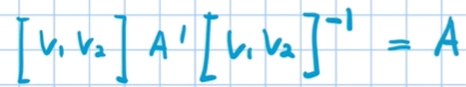
에 대해서 자세히 알아보자. 동영상에서는 위의 기저변환 일반화 공식을 이용해서 아래의 대각화 공식을 정의하고 있다.
[v1 v2] A’ [v1 v2]-1 = A’ 을 A의 고유백터 좌표를 기준으로 기저변환한 ‘결과’
[v1 v2] A’ [v1 v2]-1 = 위 ‘결과’를 다시 E를 기준으로 기저변환한 결과 = A !!
A와 A’은 위의 x1~xn, y1~yn과 같은 역할이다.
A’ 은 A의 고유값들로 만든 대각행렬, [v1 v2]는 A의 고유백터를 열백터로 가지는 행렬
A 는 [E(기본 좌표계)]를 기준좌표계(기저)로 생각하는 선형변환이다.
고민을 많이 해야하므로 위의 내용을 이해하고 싶으면 강의를 다시 보자.
이 대각화 공식을 다음과 같이 증명하면 쉽게 이해 가능하다.
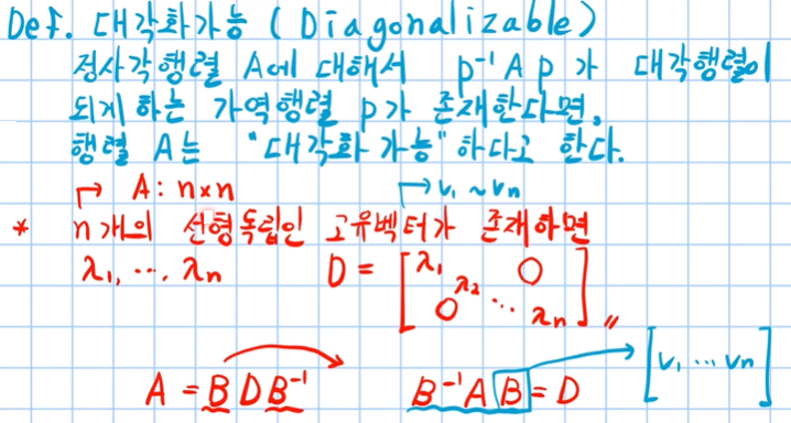
49강 대각화가능행렬과 그 성질들
대각화 가능한 행렬 A는 n개의 선형독립인 고유백터를 가진다.
n개의 선형독립인 고유백터를 가지는 A는 대각화가 가능하다.
대각화 왜해??
대각행렬(D)은 n승을 하면, 대각원소의 n승인 행렬이다.
A^n = P * D^n * inverse(P)
A^n을 대각화로 엄청 쉽게 구할 수 있다!!
50강 - 증명 : n차원에서 ‘n개의 원소를 가지는 백터 v’들의 선형독립 백터(v1 v2 … vn)의 최대갯수는 n개이다.
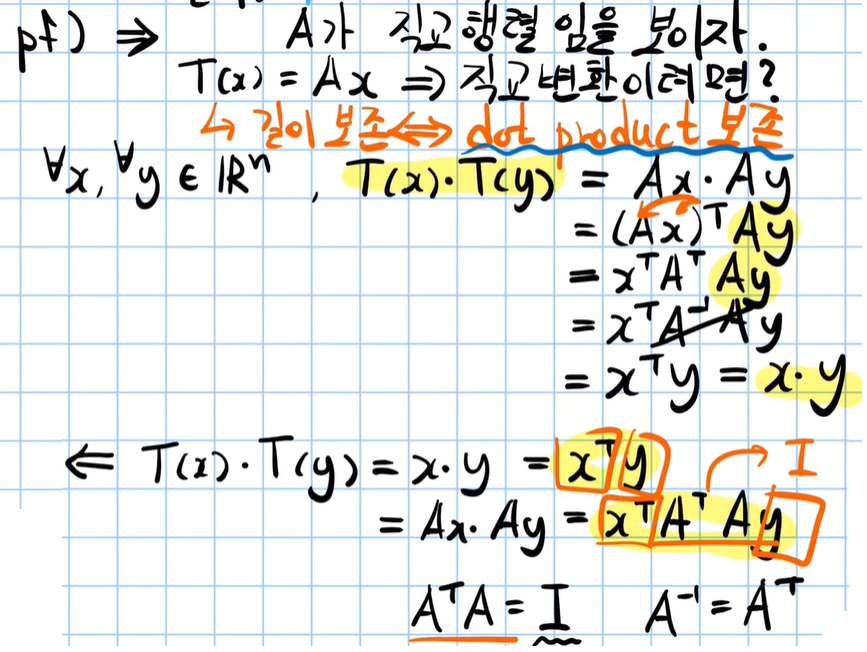
51강 - 증명 : (1) A의 span(열백터들 or 행백터들) = n이면, A는 가역행렬이다. (2) 가역행렬(n차 정사각행렬)의 행백터, 열백터는 n dimention의 기저백터(독립!, 정규일 필요 X)이다.
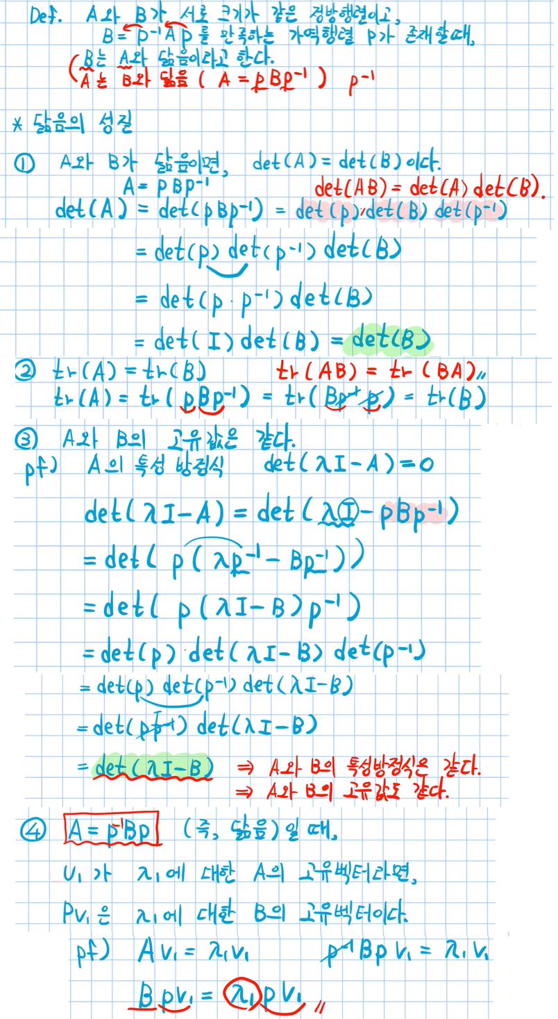
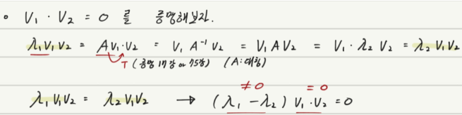
Matrix similarity, Fuctnion, Space(닮음과 함수, 공간)
52강 Matrix similarity(행렬의 닮음)
두 행렬이 서로 닮음이면, 아래와 같은 많은 성질을 가진다.
53강 kernal and range(핵과 치역)
kernal : (m x n 행렬 (n차원 백터 -> m차원 백터 로 변환하는 행렬)) 선형사상 F행렬 (=선형함수,=선형변환)에 대해, F * x = {0백터}. 즉 F에 의해서 0백터가 돼버리는 백터(n차원 공간의 좌표)들. 이 백터들을 kernal, null space(영공간) 이라고 한다.
선형사상 F에 의해서 n차원의 부분공간(원소들을 스칼라배, 덧셈을 하면 ‘집합 내의 원소’가 나오는 공간)이 m차원의 부분공간으로 변환됨
선형변환 행렬 A에 대해, range(A) (Ax의 공간. x는 백터) = col(A) (A의 colum space 차원)이다.
⭐ from이 가르키는 마지막 directory의 __init__.py 또한 일단 다 읽는다! 그리고 import다음으로 넘어간다.
우리가 아는 아주 당연한 방법으로, import 다음 내용으로 from A.B.C import py_file_name/function_defined 과 같이 import를 수행해도 된다.
하지만 from 가장 마지막 directory의 (위의 예시에서 C)의 __init__.py 안에서 한번 import된 함수를 import해서 가져와도 된다.
이를 이용해서, 궁금증2의 첫 실행문을 다시 설명하자면, from mmdet.apis 을 통해서 apis의 __init__.py를 모두 읽는다. 여기서 from .inference import (async_inference_detector, inference_detector,init_detector, show_result_pyplot) 이 수행되므로, import에서 import inference_detector, init_detector, show_result_pyplot를 하는 것에 전혀 무리가 없는 것이다.


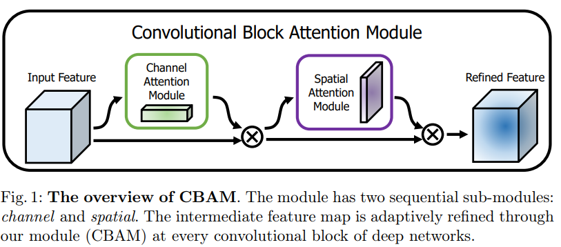


 : encodes where to emphasize or suppress.

 에 대해서 자세히 알아보자. 동영상에서는 위의 기저변환 일반화 공식을 이용해서 아래의 대각화 공식을 정의하고 있다.