【Transformer】An Image is worth 16x16 words - Image Transformers
- 논문 : An Image is worth 16x16 words : Transformers for Image Recognition at Scale
필기 완료된 파일은OneDrive\21.1학기\논문읽기에 있다. - 분류 : Transformer
- 저자 : Alexey Dosovitskiy, , Lucas Beyer , Alexander Kolesnikov , Dirk Weissenborn
- 읽는 배경 : Visoin Transformers 가 도대체 뭔지 알아보기. Attention 과 Transformer 기본 이론, 이전 Post
- 느낀점 :
- Conclution -> Method -> Introduction -> Abstract 순서로 논문을 공부하자!
- 실제 공부 순서
- Conclution -> Abstract (짧아서 이것부터 읽음)
- Methord(너무 자세하지 않다.) -> 코드 공부(내가 이해하던 그대로인데 이렇게 코딩해 놓다니 예술이다)
- 유투브 동영상 보기 (동영상 링크)
- 논문 나머지 공부하기
- 목차

(gif 출처 : https://github.com/lucidrains/vit-pytorch)
<Vision Transformer paper>
0. Conclusion, Abstract
- Transformers to image recognition 을 수행해보았다.
- 지금까지 다른 논문들은, Computer vision에서 self-attention을 사용했다. self-attention을 하기 위해서 다른 논문들은 inductive biases into the architecture (전체 Network에 attention module을 따로 설치한 행위를 의미하는 듯) 을 적용했지만, 우리는 그러지 않았다.
- CNN에 의존하는 방식이 아니라, Pure transformer 방식을 적용했다. classification을 잘 수행하는 것을 확인했고, CNN이 필수적이 아니라는 것도 확인했다.
- Image sequence of Patches 를 NLP에서 사용하는 Transformer encoder에 넣었다.
- classification 과제 (ImageNet, CIFAR-100, VTAB, etc.) 에서 SOTA를 달성했고, 다른 모델에 비해 가볍다.
- many challenges 남아있다.
- detection and segmentation 으로 나아가야한다. “End-to-end object detection with transformers” 를 거론하고 있다.
- self-supervised training methods 에 대한 탐구가 더 이뤄져야한다. - Our initial 실험에는 self-supervised pre-training을 사용해서 성능 향상을 이루었다. 하지만 self-supervised 만으로는 supervised 를 이길 수 없었다.
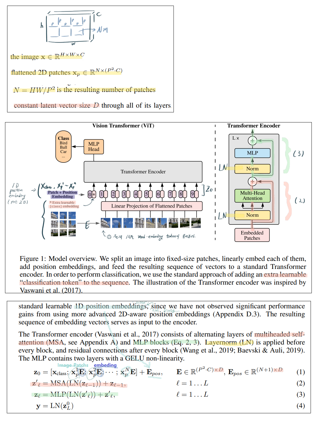
2. Method
original Transformer (Vaswani et al., 2017) 를 최대한 따르려고 노력했다. (그래서 이 논문에서는 original Transformer “Attention is all you need.” 에 나오는 내용은 추가로 설명하지 않는다. 그래서 이 논문이 어렵다. “Attention is all you need.”논문의 내용은 대강 아는데, (논문을 훑어 봐도 이전 Post 내용 이외에 특별한 내용은 없다. 결국에 코드를 봐서 이해하는게 필요하다.) )
논문에 나오는 내용을 아래와 같이 최종 정리 해놓았다. 이해가 안되는 건, 논문에도 안 써 있다. 결국엔 코드를 봐야한다. 코드를 보자.
(코드 내용 추가) 아래 이미지 사이즈에서, h = w = image_size 이며, h=w는 p로 나누어 떨어져야한다.
(코드 내용 추가) 특히 아래 Position Embeding은 sin을 사용하지 않고, nn.parameter를 사용해 그냥 learnable 변수로 정의했다. Class embeding 또한 nn.parameter를 사용해 그냥 learnable 변수로 정의했다.
Hybrid Architecture
- 위에서는 원본 이미지를 patch로 나눈 후, 1차원 백터로 Embeding을 해서 Transformer에 그대로 넣는 방식를 취했었다.
- (PS) Positional embeding 값도 똑같이 1차원이여야한다. 이 값은 original Transformer 논문 처럼 sin함수를 사용해도 되고, learnable parameter를 사용해도 된다. 아래의 코드에서는 learnable parameter를 사용했다.
- 하지만! CNN으로 Feature Map을 일부 뽑아내고, 그렇게 뽑아낸 Feature를 Transformer에 넣는 방식은 어떨까? 이 방식을 사용한 것이 Hybrid Architecture 이다.
- 아래에 실험결과가 나와있지만, 결과는 학습초반에는 좀 더 좋은 성능을 보이다가, 후반에 많은 데이터로 학습 시키고 나서는 1번의 일반 Transformer를 사용한 것이 더 좋은 성능을 보여주었다.
3. Experiments and Results
- 읽지는 않겠다.
- 필요하면 그때 찾아 읽자.
- Youtube 발표자료 부분에 간략히 정리되어 있기도 하다.
<Vision Transformer - Pytorch code>
- 원래 논문의 code 는 이 사이트(google-research/vision_transformer) 이다.
- Pytorch vit 코드 링크 https://github.com/lucidrains/vit-pytorch
- 하지만 이 코드는 flax, vit_jax 라는 새로은 딥러닝 프레임워크를 사용한다. 이 프레임워크는 tensorflow2.0이 망할 것 같아서 구글이 새로 내놓은 프레임워크 같다. 옛날에 Raddit을 통해서, pytorch vs tensorflow vs falx+vit_jax 에 대해서 검색해 본 결과, 대충 결론은 이랬다. “tensorflow 1.3으로 나왔던 코드들은 tensorflow 2.0으로 다시 만들어 지지않는다. 최근 논문들도 대부분 pytorch를 사용한다. 구글에서 만든 것이 항상 최고는 아니다. falx+vit_jax 를 구글에서 새로 만들어 발표하기는 했지만, 이게 어떻게 될지는 아무도 모른다”
- 앞으로 내가 살면서 Pytorch는 영원하지 않다. 개발자는 개발 언어에 큰 비중을 두어서는 안된다. 영원할 것만 같은 개발 언어도 언젠간 망하기 마련이고, 개발자는 그 변화에 빠르고 신속하게 적응해야한다. 개발자는 코딩의 전반적 지식과, 알고리즘, 그리고 논문 지식을 통해서 능력을 발휘할 수 있다.
- 아이러니 하게도, flax, vit_jax 로 만들어진 vit (vision transformer) 코드는 1.8k stars를 가지고 있고, pytorch로 만들어진 vit 코드는 2.8k이다. 원래 것 보다 더 높은 star를 가지고 있다.
Colab 환경세팅
from google.colab import drive
drive.mount('/content/drive')
%cd /content/drive/MyDrive/GCPcode/torch_package
!ls

# !git clone https://github.com/lucidrains/vit-pytorch.git
%cd vit-pytorch
!python setup.py install

# no module einops 문제 해결방법
!pip install einops==0.2.0
!pip install einops==0.3.0
- vision transformer 에는 몇가지 사용방법이 존재한다.
- 16x16 Image recognition 논문에서 사용한 방법이 아래 1번의 방법이다.
- 나머지 2번 ~ 5번의 방법은, 다른 논문에서 소개된 방법론이다. 이것까지 코드로 어떻게 사용하는지 소개해 놓았다.
- from vit_pytorch import ViT
- from vit_pytorch.t2t import T2TViT
- SOTA self-supervised learning technique : from vit_pytorch import ViT + from byol_pytorch import BYOL
- Efficient Attention : Nystromformer (computer vision cost(메모리,시간)를 낮춰주는 새로운 방법)
- x-transformers : used the most vanilla of attention networks
- 따라서, 일단 나는, 16x16 Image recognition 논문을 먼저 이해하고 싶으므로, 위의 1번의 방법만 잘 이해하면 된다.
- 위 1번 방법의 코드는
vit-pytorch/vit_pytorch/vit_pytorch.py여기있는게 전부이다.
코드 리뷰
- 핵심 코드 https://github.com/lucidrains/vit-pytorch/blob/main/vit_pytorch/vit_pytorch.py
- 아래의 코드 내부 주석에 소중한 내용들이 많이 들어갔으니 꼭 참고하기!!
from einops import rearrange, repeat이라는 마법의 이미지 변환 모듈을 사용했다.from torch import einsum이라는 마법의 텐서 변환 모듈을 사용했다.- 위의 2 모듈은
string을 입력하면 그 문자에 맞추어, 배열을 변환해 준다. - 예를 들어 이렇게
Rearrange("b c (h p1) (w p2) -> b (h w) (p1 p2 c)", p1 = patch_size, p2 = patch_size)
- 위의 2 모듈은
- 실행 코드
import torch
from vit_pytorch import ViT

v = ViT(
    image_size = 256,
    patch_size = 32,
    num_classes = 1000,
    dim = 1024, # A image patch가 변환되어, 1차원 백터가 됐을 때, 백터 원소의 갯수
    depth = 6, # Transformer blocks 갯수 ( Transformer Encoder 그림에서 x L )
    heads = 16, # heads in Multi-head Attention layer 의 갯수
    mlp_dim = 2048, # Multi Layer perceptron 에서 0층 1층 2층에서 1층의 백터 갯수
    dropout = 0.1, # [0,1] 사이의 수. default = 0
    emb_dropout = 0.1
)

img = torch.randn(1, 3, 256, 256)
mask = torch.ones(1, 8, 8).bool() # optional mask, designating which patch to attend to

preds = v(img, mask = mask) # (1, 1000)
- class ViT(nn.Module)
class ViT(nn.Module):
    def __init__(self, *, image_size, patch_size, num_classes, dim, depth, heads, mlp_dim, pool = 'cls', channels = 3, dim_head = 64, dropout = 0., emb_dropout = 0.):
        super().__init__()
        assert image_size % patch_size == 0, 'Image dimensions must be divisible by the patch size.'
        num_patches = (image_size // patch_size) ** 2 # ( 224/32 = 16 ) ** 2 = 256의 Patchs
        patch_dim = channels * patch_size ** 2  # patch 하나가 가진 pixel의 총 갯수 = 32*32*3 = 3072
        assert pool in {'cls', 'mean'}, 'pool type must be either cls (cls token) or mean (mean pooling)'

        # from einops import rearrange, repeat 이라는 마법의 이미지 변환 모듈 사용
        # 아래의 과정을 통해서 이미지를 1차원 dim
        self.to_patch_embedding = nn.Sequential(
            Rearrange('b c (h p1) (w p2) -> b (h w) (p1 p2 c)', p1 = patch_size, p2 = patch_size),
            nn.Linear(patch_dim, dim), # 3072 -> 1024
        )

        # sin 함수를 이용한 embedding을 하는 줄 알았는데...
        # randn 은 그냥 원하는 크기의 Tensor를 설정해줄 뿐, Parameter로 세팅해놓음으로써, Learnable이 된다.
        # 즉 pos_embedding 그리고 cls_token 는 Just Tensor가 아니라 Learnable 이다.
        self.pos_embedding = nn.Parameter(torch.randn(1, num_patches + 1, dim))
        self.cls_token = nn.Parameter(torch.randn(1, 1, dim))
        self.dropout = nn.Dropout(emb_dropout)

        # Transformer Encoder layer 정의
        self.transformer = Transformer(dim, depth, heads, dim_head, mlp_dim, dropout)

        self.pool = pool  # string in {'cls', 'mean'}
        self.to_latent = nn.Identity()

        # layerNorm 이라는게 있나보다. 그냥 mlp_head는 nn.Linear 라고 생각하면 편하다.
        self.mlp_head = nn.Sequential(
            nn.LayerNorm(dim),
            nn.Linear(dim, num_classes) # 1024 -> 1000
        )

    def forward(self, img, mask = None):
        x = self.to_patch_embedding(img)
        b, n, _ = x.shape

        cls_tokens = repeat(self.cls_token, '() n d -> b n d', b = b)
        x = torch.cat((cls_tokens, x), dim=1)
        x += self.pos_embedding[:, :(n + 1)]
        x = self.dropout(x)

        x = self.transformer(x, mask)
        # print(x.shape) # torch.Size([1, 65, 1024])

        x = x.mean(dim = 1) if self.pool == 'mean' else x[:, 0]
        # print(x.shape) # torch.Size([1, 1024])

        x = self.to_latent(x)
        out = self.mlp_head(x)
        # print(out.shape) # torch.Size([1, 1000])
        return out

"""
여기서 알아야 하는 것.
nn.LayerNorm(dim)
nn.Identity()
class Transformer(nn.Module):
"""
- class Transformer(nn.Module):
- 논문 그림에서 “Transformer Encoder” 를 그대로 코드 구현을 해 놓은 것이다.
class Transformer(nn.Module):
    def __init__(self, dim, depth, heads, dim_head, mlp_dim, dropout = 0.):
        super().__init__()
        self.layers = nn.ModuleList([])
        for _ in range(depth):
            self.layers.append(nn.ModuleList([
                Residual(PreNorm(dim, Attention(dim, heads = heads, dim_head = dim_head, dropout = dropout))),
                Residual(PreNorm(dim, FeedForward(dim, mlp_dim, dropout = dropout)))
            ]))
    def forward(self, x, mask = None):
        for attn, ff in self.layers:
            x = attn(x, mask = mask)  # LayerNorm + Attention   + Residual
            x = ff(x)			      # LayerNorm + FeedForward + Residual
        return x

"""
여기서 알아야 하는 것.
Residual
PreNorm
FeedForward
Attention
"""
- class Residual : Skip connection 구현
- class PreNorm : LayerNorm + [FeedForward or Attention]
- class FeedForward : Multi Layer perceptron = 2층 nn.Linear
class Residual(nn.Module):
    # Skip connection 구현
    def __init__(self, fn):
        super().__init__()
        self.fn = fn # 무조건 class PreNorm
    def forward(self, x, **kwargs):
        return self.fn(x, **kwargs) + x


class PreNorm(nn.Module):
    # LayerNorm + [FeedForward or Attention]
    def __init__(self, dim, fn):
        super().__init__()
        self.norm = nn.LayerNorm(dim)
        self.fn = fn  # class FeedForward 혹은 class Attention 둘 중 하나
    def forward(self, x, **kwargs):
        x = self.norm(x)
        return self.fn(x, **kwargs)


class FeedForward(nn.Module):
    # Multi Layer perceptron = 2층 nn.Linear
    def __init__(self, dim, hidden_dim, dropout = 0.):
        super().__init__()
        self.net = nn.Sequential(
            nn.Linear(dim, hidden_dim),
            nn.GELU(),
            nn.Dropout(dropout),
            nn.Linear(hidden_dim, dim),
            nn.Dropout(dropout)
        )
    def forward(self, x):
        return self.net(x)
- class Attention(nn.Module) : Multi Head Attention 모듈 구현
- 아래에서 Keys, Querys, Values가 의미하는게 뭘까? 이전Post 내용에 따르면, 1차원 백터에서 어떤 부분에 더 집중해야 하는지? 를 나타낸다고 한다.
- 아래의
qkv = self.to_qkv(x).chunk(3, dim = -1)에서 x는 이미지 전체를 1차원 백터(1024개)로 embeding한 값들이 8*8 (64개 patchs)가 모두 모여 있는 백터이다. 즉, 1024 x 64의 x.shape를 가지고 있을 것이다. - 자, 그렇다면 64개의 patch 하나하나를 하나의 단어라고 생각하자.
- 이전Post 내용에 따르면 “Hello I love you”에서 Love는 I와 you에 더 attention해야하고, 따라서 더 큰 weight를 줘야한다.
- 같은 원리로 64개의 patch 각각에 대해서, 1개의 Patch는 다른 patch 중 어느 것에 더 집중해서 attention해야하는지를 weight값으로 알려주는 것이 Keys, Querys, Values이고, 이 처리를 모두 하고 나온 백터가 qkv이다.
class Attention(nn.Module):
    def __init__(self, dim, heads = 16, dim_head = 64, dropout = 0.):
        '''
        dim = patch를 1차원화 백터 원소의 갯수 = 1024 개
        heads = 1, 2, 3 ... ~ h (Multi-head Attention)에서 h 갯수

        처음 들어가는 1개 image patch의 차원 [1, 1024]
        [x1 ~ x65] = [1, 65, 64] # 원래 patch갯수는 64개 + extra class embedding 1개 = 65개
        하나의 Head에 의해 나오는 y_i의 차원 [1, 64]
        [y1 ~ y65] = [1, 65, 64]
        '''
        super().__init__()
        inner_dim = dim_head *  heads # 64*16 = 1024
        project_out = not (heads == 1 and dim_head == dim)

        self.heads = heads
        self.scale = dim_head ** -0.5 # 0.125
		"""
        # qkv의 nn.linear 를 그림처럼 따로 하는게 아니라, 한꺼번에 해버린다.
        # 아래의 *3 이 의미하는 것은 qkv 3개를 말하는 건가?
        # inner_dim 은 qkv 중 하나의 linear를 통과했을 때 나오는 총 원소의 갯수
        # 즉 dim_head는 위 Transformer 이미지에서, 하나의 작은 linear를 통과했을 때 나오는 원소의 갯수 이다.

        # input은  queries, keys, values와 연산되어 (nn.linear), forward 코드와 같이 각각 q, k, v 변수가 된다.
        # by queries : (input)1024 vectors -> 64 vectors * 16개 head
        # by keys : 1024 vectors -> 64 vectors * 16개 head
        # by values : 1024 vectors -> 64 vectors * 16개 head
        """
        self.to_qkv = nn.Linear(dim, inner_dim * 3, bias = False)

        self.to_out = nn.Sequential(
            nn.Linear(inner_dim, dim), # (64*16 = 1024) -> 1024개
            nn.Dropout(dropout)
        ) if project_out else nn.Identity()

    def forward(self, x, mask = None):
        """
        # heads의 갯수 설정으로 내부에서 다수의 head가 알아서 돌아간다.
        # 주의! heads는 Transformer Encoder의 Lx에서 L이 아니다! 맨 위 사진의 1~h에서 h 이다!
        # 따로 분류해서 연산하지 않고, 한꺼번에 묶어서 연산해 버린다.
        # 그래서 이 코드로는 위 그림의 이해가 한방에 되지 않을 수 있다.

        # 따라서 아래 내용이 복잡하지만... "이거 다 통과하면 하나의 Multi Head Attention 을 통과하는 구나! 라고 알아두자."
        """

        b, n, _, h = *x.shape, self.heads
        # print(x.shape) # torch.Size([1, 65, 1024])
        qkv = self.to_qkv(x).chunk(3, dim = -1)
        # print(qkv.shape, qkv[0].shape) # (3,) torch.Size([1, 65, 1024])
        # torch.chunk Tensor를 자른다.
        # q, k, v 각각, input에서 by queries, keys, values 처리를 하고 나오는 '결과'
        q, k, v = map(lambda t: rearrange(t, 'b n (h d) -> b h n d', h = h), qkv)
        # print(q.shape,k.shape,v.shape) # torch.Size([1, 16, 65, 64]) torch.Size([1, 16, 65, 64]) torch.Size([1, 16, 65, 64])

        # torch.einsum (https://pytorch.org/docs/stable/generated/torch.einsum.html)
        # tensor를 원하는 형태로 변환해줘!
        dots = einsum('b h i d, b h j d -> b h i j', q, k) * self.scale
        mask_value = -torch.finfo(dots.dtype).max

        if mask is not None:
            mask = F.pad(mask.flatten(1), (1, 0), value = True)
            assert mask.shape[-1] == dots.shape[-1], 'mask has incorrect dimensions'
            mask = rearrange(mask, 'b i -> b () i ()') * rearrange(mask, 'b j -> b () () j')
            dots.masked_fill_(~mask, mask_value)
            del mask

        attn = dots.softmax(dim=-1)

        out = einsum('b h i j, b h j d -> b h i d', attn, v)
        """
        여기까지 out = torch.Size([1, 16, 65, 64])
        <맨 위의 Transformer 최종 정리 사진과 꼭 함께 보기>
        이 말은 하나의 Head에 의해 나오는 y_i는 64개의 백터를 가진다. 총 [y1 ~ y65] = [1, 65, 64] 차원을 가지게 된다.
        """
        out = rearrange(out, 'b h n d -> b n (h d)')
        out =  self.to_out(out)
        # print(out.shape) # torch.Size([1, 65, 1024])
        return out
Youtube 발표자료
- Youtube Link 한국어 : https://www.youtube.com/watch?v=D72_Cn-XV1g
- Youtube Link 영어 : https://www.youtube.com/watch?v=TrdevFK_am4&t=847s - 필요하면 이 자료가 더 좋을 듯 하다.
- 강의 자료 필기본 Github 저장소
- 총 23장의 pdf 이미지가 있지만, 아래에는 유용한 자료만 남겨놓았다. 하지만.. Experience Setup 과 Result 부분만 조금 참고하면 좋을 듯 하지만, 굳이 안봐도 되기도 하다. 유튜브 영상과 발표 자료의 질이 그렇게 좋은 편은 아닌듯 하다.
![]()
![]()

- Method는 내가 한 정리가 더 좋다.
- Experiments and Results
![]()
![]()
![]()
![]()
![]()
![]()
![]()
![]()
![]()