【ClassBlance】Large-Scale Long-Tailed Recognition in an Open World = OLTR w/ advice

26 Jan 2021 in Artificial Intelligence

• 논문 : Large-Scale Long-Tailed Recognition in an Open World - y2019-c103
• 분류 : Unsupervised Domain Adaptation
• 저자 : Ziwei Liu1,2∗ Zhongqi Miao2∗ Xiaohang Zhan1
• 읽는 배경 : (citation step1) Open Componunt Domain Adaptation에서 Memory 개념이 이해가 안되서 읽는 논문.
• 읽으면서 생각할 포인트 : 논문이 어떤 흐름으로 쓰여졌는지 파악하자. 내가 나중에 쓸 수 있도록.
• 동영상 자료
  • 
• 질문
  • centroids메모리 M을 어떻게 학습시키는지는 아직 모르겠다. 이것은 코드를 통해서 공부하면 될듯.
    OLTR/models/MetaEmbeddingClassifier.py 파일에 forward의 input으로 centroids가 들어가는 것을 확인할 수 있다.
• 선배님 조언
  • 외국에서 사는게 그리 좋은게 아니다. 우리나라 라는 것이 얼마나 큰 축복인지 모른다. 기회가 있다면 나가서 일하고 나중에 다시 돌아오면 된는거다. 우리나라에 대해서 감사함을 가지고 살아가도록 해야겠다.
  • 특히나 외국에서 오래 살고 오셨기 때문에, 저 진심으로 해주시는 조언이었다. 그냥 큰 환상을 가지고 거기서 살고 싶다 라는 생각을 해봤자 환상은 깨지기 마련이고, 우리나라 안에서, 우리나라가 주는 편안함과 포근함에 감사하며 살아가는게 얼마나 큰 축복인지 알면 좋겠다. 모비스와 다른 외국 기업과의 비교를 생각하며 감사할 줄 몰랐다. 하지만 감사하자. 모비스에 가서도 정말 열심히 최선을 다해, 최고가 되기 위해 공부하자. 그렇게 해야 정말 네이버든 클로버든 갈 수 있다. 그게 내가 정말 가야할 길이다. 그러다가 기회가 되어 외국 기업이 나를 부른다면, 다녀오면 된다. 그리고 또 한국이 그리워지면 다시 돌아오면 되는거다. 나의 미래를 좀 더 구체적으로 만들어 주신 선배님께 감사합니다.
  • 학교에서 너무 많은 것을 배우려고 하지 마라. 수업은 그냥 쉬운게 짱. 하고 싶은 연구하고 하고 싶은 공부하는게 최고다. 그리고 동기와 친구와 같이 수업 듣는 것을 더 추천한다.

느낀점

1. Instruction이 개같은 논문은..
   • abstract 빠르게 읽고, Introduction 대충 읽어 넘겨야 겠다. 뭔소리하는지 도저히!!!!!! 모르겠다.
   • 지내들이 한 과정들을 요약을 해놨는데.. 나는 정확히 알지도 못하는데 요약본을 읽으려니까 더 모르겠다.
   • 따라서 그냥 abstract읽고 introduction 대충 모르는거 걍 넘어가서 읽고.
   • relative work의 새로운 개념만 빠르게 훑고, 바로 Ours Model에 대한 내용들을 먼저 깊게 읽자. 그림과 함께 이해하려고 노력하면서.
   • 그리고! Introduce을 다시 찾아가(👋) 읽으며, 내가 공부했던 내용들의 요약본을 읽자
2. 아무리 Abstract, Instruction, Relative work를 읽어도, 이해가 되는 양도 정말 조금이고 머리에 남는 양도 얼마 되지 않는다. 지금도 위 2개에서 핵심이 뭐였냐고 물으면, 대답 못하겠다.
   • 현재의 머신러닝 논문들이 다 그런것 같다. 그냥 대충 신경망에 때려 넣으니까 잘된다.
   • 하지만 그 이유는 직관적일 뿐이다. 따라서 대충 이렇다저렇다 삐까뻔쩍한 말만 엄청 넣어둔다. 이러니 이해가 안되는게 너무나 당연하다.
   • 이런 점을 고려해서, 좌절하지 않고 논문을 읽는 것도 매우 중요한 것 같다. (👋)여기 아직 안읽었다고??? 걱정하지 마라. 핵심 Model 설명 부분 읽고 오면 더 이해 잘되고 머리에 남는게 많을거다. 화이팅.
3. 확실히 Model에 더 집중하니까, 훨씬 좋은 것 같다. 코드까지 확인해서 공부하면 금상첨화이다. 이거 이전에 읽은 논문들은, 그 논문만의 방법론에는 집중하지 못했는데, 나중에 필요하면 꼭! 다시 읽어서 여기 처럼 자세히 정리해 두어야 겠다.
4. 이 논문의 핵심은 이미 파악했다. 👋 읽기 싫다. 안 읽고 정리 안했으니, 나중에 필요하면 참고하자. 명심하자. 읽을 논문은 많다. 모든 논문을 다 정확하게 읽는게 중요한게 아니다.

0. Abstract

• the present & challenges
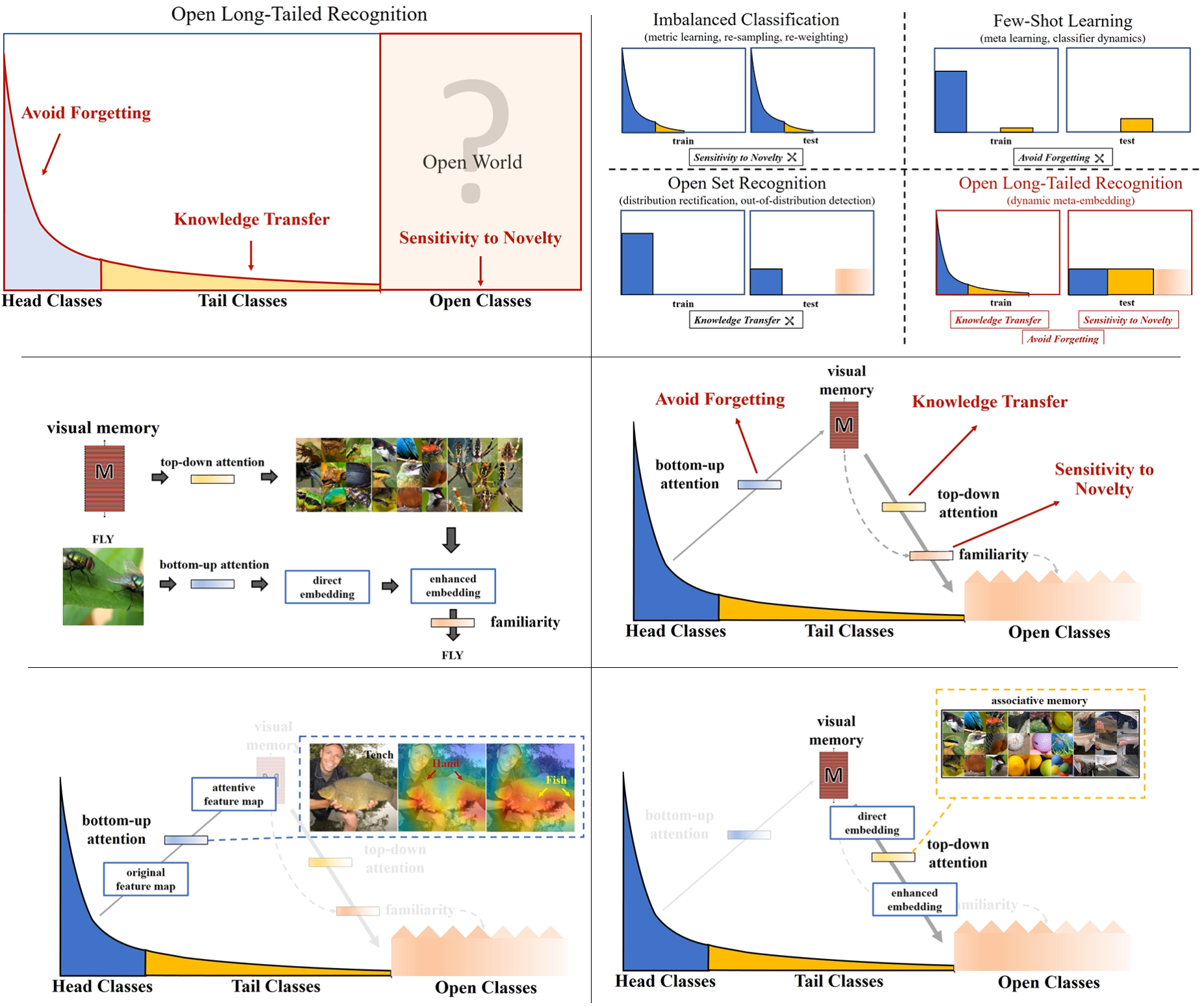
  1. Real world data often have a long-tailed and open-ended distribution. 즉 아래의 그래프의 x축은 class종류를 데이터가 많은 순으로 정렬한 것이고, y축은 해당 클래스를 가지는 데이터 수. 라고 할 수 있다. Open Class는 우리가 굳이 Annotate 하지 않는 클래스이다.
  2. 
• Ours - 아래 내용 요약

1. Introduction

• the past
  • 대부분의 기법들은 Head Class 인식에 집중하지만,
    최근 Tail class 문제를 해결하기 위한 방법이 존재한다. (=Few-shot Learning)for the small data of tail classes [52, 18]
• Ours

  • 우리의 과제(with one integrated algorithm)
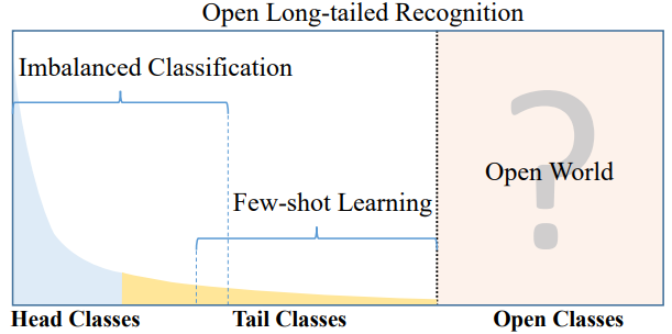
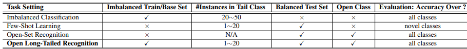
    1) imbalanced classification
    2) few-shot learning
    3) open-set recognition
    즉. tail recognition robustness and open-set sensitivity:

  • Open Long-Tailed Recognition(OLTR) 이 해결해야하는 문제
    1) how to share visual knowledge(=concept) between head and tail classes (For robustness)
    2) how to reduce confusion between tail and open classes (For sensitivity)

  • 해결방법

    • 2번째 페이지 We develop an OLTR 문단부터 너무 이해가 어렵다. 따라서 일단 패스하고 다시 오자. 요약본이니, 구체적으로 공부하고 나면 이해하기 쉬울 거다. 👋

    • # 이전에 정리해 놓은 자료. 나중에 와서 다시 참조.
      1 mapping(=dynamic meta-embedding) an image to a feature space  = **a direct feature** computed(embeded) from the input image from the training data   
      2) visual concepts(=visual memory feature) 이 서로서로 연관된다.(associate with) = A visual memory holds **discriminative centroids**     
      3) A summary of **memory activations** from the direct feature   
      그리고 combine into a meta-embedding that is enriched particularly for the tail class.
      

  • .

  # 2. Related Works

  

• Imbalanced Classification

  • Classical methods - under-sampling head classes, over-sampling tail classes, and data instance re-weighting.
  • Some recent methods - metric learning, hard negative mining, and meta learning.
  • Ours
    • combines the strengths of both metric learning[24, 37] and meta learning[17, 59]
    • Our dynamic meta-embedding~~~ 👋

• Few-Shot Learning

  • 초기의 방법들 they often suffer a moderate performance drop for head classes.
  • 새로운 시도 : The few-shot learning without forgetting, incremental few-shot learning.
  • 하지만 : 위의 모든 방법들은, the training set are balanced.
  • In comparison, ours~~~ 👋

• Open-Set(new data set) Recognition

  • OpenMax [3] : calibrating the output logits
  • OLTR approach incorporates~~ 👋

3. Our OLTR Model

• 우리 모델의 핵심은 Modulated Attention 그리고 Dynamic meta-embedding 이다.
  • dynamic Embedding : visual concepts(transfers knowledge) between head and tail
  • modulated Attention : discriminates(구분한다) between head and tail
  • reachability : separates between tail and open
• Our OLTR Model
  • We propose to map(mapping하기) an image to a feature space /such that visual concepts can easily relate to each other /based on a learned metric /that respects the closed-world classification /while acknowledging the novelty of the open world.

3-1. Dynamic Meta-Embedding

• combines a direct image feature and an associated memory feature (with the feature norm indicating the familiarity to known classes)

  • CNN feature 추출기 가장 마지막 뒷 단이 V_direct(linear vector=direct feature)이다. (classification을 하기 직전)
  • tail classes(data양이 별로 없는 class의 데이터)에는 사실 V_direct이 충분한 feature들이 추출되어 나오기 어렵다. 그래서 tail data와 같은 경우, V_memory(memory feature) 와 융합되어 enrich(좀더 sementic한 정보로 만들기) 된다. 이 V_memory에는 visual concepts from training classes라는게 들어가 있다.

• Learning Visual Memory (M)

  • [23] 이 논문의 class structure analysis and adopt discriminative centroids 내용을 따랐다.
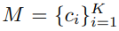  • 여기서 K는 class의 갯수이다.
  • M은 V_direct에 의해서 학습이 된다. centroids 정보가 계속적으로 Update된다고 한다. 여기서 centroids정보는 아래의 삼각형 위치이다. 아래의 작은 동그라미가 V_direct 정보이고, 그것의 중심이 centroids가 된다.
  • 이 centroids는 inter-class에 대해서 거리가 가장 가깝게, intra-class에 대해서는 거리가 최대한 멀게 설정한다.
  • 
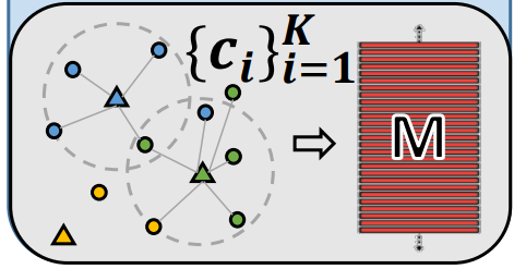
  • centroids를 어떻게 계산하면 되는지는 코드를 좀만 더 디져보면 나올 듯하다. 아래 python코드의 centroids가 핵심이다. centroids는 model의 forward 매개변수로 들어온다.

• Memory Feature (V_memory)

  • O : V_direct와 i번째 클래스간의 상관계수(coefficients hallucinated(상관관계라고 환각이 느껴지는 단순한 Fully Conected Layer….))를 의미한다.

  • V_memory는 아래의 코드처럼 M과 O를 torch.matmul해서 만들어 낸다.

  • Github Link

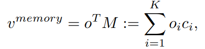
    • # set up visual memory . [M 만들기]
      x_expand = x.clone().unsqueeze(1).expand(-1, self.num_classes, -1)
      centroids_expand = centroids.clone().unsqueeze(0).expand(batch_size, -1, -1)
      keys_memory = centroids.clone()
            
      # computing reachability
      dist_cur = torch.norm(x_expand - centroids_expand, 2, 2)
      values_nn, labels_nn = torch.sort(dist_cur, 1)
      scale = 10.0
      reachability = (scale / values_nn[:, 0]).unsqueeze(1).expand(-1, feat_size)
            
      # computing memory feature by querying and associating visual memory
      # self.fc_hallucinator = nn.Linear(feat_dim, num_classes)
      values_memory = self.fc_hallucinator(x.clone())
      values_memory = values_memory.softmax(dim=1)
      memory_feature = torch.matmul(values_memory, keys_memory)
      

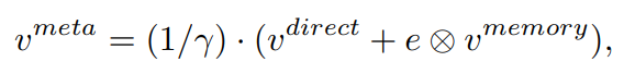
• V_meta

  • 
  • V_meta이 정보가 마지막 classifier에 들어가게 된다.
  • 
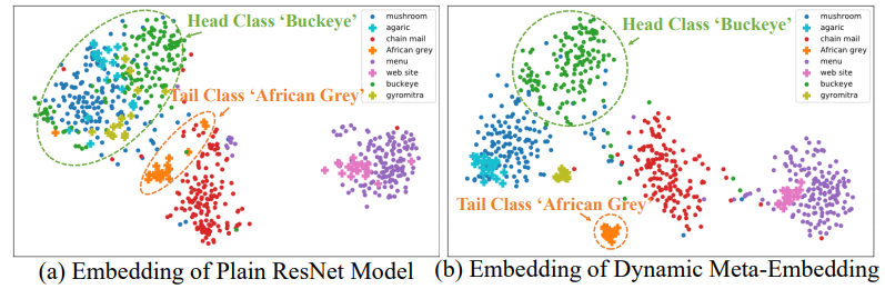
  • 왼쪽 이미지 처럼, 그냥 V_direct를 사용하면, inter-class간의 거리가 멀리 떨어지는 경우도 생긴다.
  • 오른쪽 그림은, V_meta를 확인한 것인데, inter-class간의 거리가 더 가까워진 것을 확인할 수 있다.

• Reachability (γ)

  • closed-world class에 open-world class를 적용하는데 도움을 준다.
  • 공식은 이와 같고,
  • 이것이 의미하는 바는, class 중에서 어떤 class의 centroids와 가장 가까운지 Open-world data의 V_direct와 비교를 하는 것이다. 가장 가까운 class에 대해서(γ 작음) V_meta에 큰 값을(1/γ큼) 곱해 주게 된다.
  • 이것은, encoding open classes를 사용하는데에 더 많은 도움을 준다.

• e (concep selector)

  • head-data의 V_direct는 이미 충분한 정보를 담고 있다. tail-data의 V_direct는 상대적으로 less sementic한 정보를 담고 있다.
  • 따라서 어떤 데이터이냐에 따라서 V_memory를 사용해야하는 정보가 모두 다르다. 이런 관점에서 e (nn.Linear(feat_dim, feat_dim)) 레이어를 하나 추가해준다.
  • 따라서 e는 다음과 같이 표현할 수 있다.

• dynamic meta-embedding **facilitates feature sharing** between head and tail classes

3-2. Modulated Attention

• Modulated attention : encourages different classes to use different contexts(attentions), which helps maintain the discrimination between head and tail classes.
  • 
• V_direct를 head와 tail class 사이, 그리고 intra-class사이의 차이를 더 크게 만들어 주는 모듈이다. 위의 이미지에서 f가 f^(att)가 되므로써, 좀 더 자신의 class에 sementic한 feature를 담게 된다. 이 attention모듈을 사용해서 f에 spatial and different contexts를 추가로 담게 된다.
• 아래의 Attention 개념은 논문이나, 코드를 통해 확인
  • SA : self-correlation, contextual information [56]
  • MA : conditional spatial attention [54]
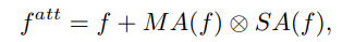• 여기서 f는 CNN을 통과한 classifier들어가기 바로 전.
• 이 개념은 다른 어떤 CNN모듈에 추가해더라도 좋은 성능을 낼 수 있는 flexible한 모듈이라고 한다.

3.3 Learning

• cosine classifier [39, 15]를 사용한다. 해당 논문 2개는 few-shot 논문이다.
• 이 방법은 아래의 방법을 사용하는 방법이다. V_meta와 classifier의 weight까지 normalize한다.
  • 
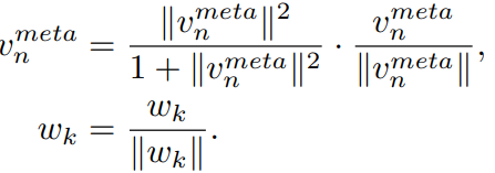
  • 이러한 normalize에 의해서, vectors of small magnitude는 더 0에 가까워지고, vectors of big magnitude는 더 1에 가까워 진다. the reachability γ 와 융합되어 시너지 효과를 낸다고 한다.

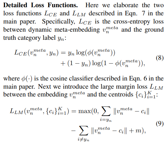
3.4 Loss function

• 
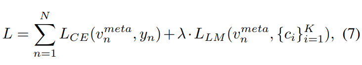
• cross-entropy classification loss, large-margin loss
• 내 생각. 위 식의 v^meta는 classification이 된 결과를 말하는 것일 것이다. vector_meta가 아니라.
• 오른쪽 loss항을 통해서, the centroids {ci} K i=1 를 학습 시킨다.
• 자세한 loss 함수는 부록 참조
  • 

4. Experiments

1. Datasets
   • Image-Net2012를 사용해서 head와 tail을 구성시킨다. 115.8k장의 이미지. 1000개의 카테고리. 1개의 카테고리에 최대 이미지 1280개, 최소 이미지 5개로 구성한다.
   • Openset은 Image-Net2010을 사용하였다.
2. Network Architecture - ResNet 사용
3. Evaluation Metrics
   • the closed-set (test set contains no unknown classes)
   • the open-set (test set contains unknown classes)
   • Train을 얼마나 반복해서 시켰는지에 따라서, many-shot classes / medium-shot classes / few-shot classes를 기준으로 accuracy를 비교해 보았다.
   • For the open-set setting, the F-measure is also reported for a balanced treatment of precision and recall following [3]. (혹시 내가 Open-set에 대한 accuracy 평가를 어떻게 하는지 궁금해 진다면 이 measure에 대해서 공부해봐도 좋을 듯 하다.)
4. Ablation Study / Result Comparisons / Benchmarking results