【DG】 Survey DG papers 6 - recent papers

25 Oct 2021 in Artificial Intelligence

• DG survey

High Level 정리

1. (#5.3) Test-Time Adaptation to Distribution Shift by Confidence Maximization and Input Transformation
   • TENT에서 무엇을 개선한건가? 무엇을 맘에 안들어 하는 것인가?
     1. Entropy Loss의 2가지 문제점 (1) dominant class prediction / (2) high confidence Gradient vanishing
     2. Domain shift가 강한 Target 이미지를 그대로 Input으로 사용하는 것
   • 사용한 해결 방안
     1. Class distribution matching loss
     2. Cross Entropy → Negative log likelihood
     3. Image Transformation = Undo domain shift
2. (#6.1) S4T: Source-free domain adaptation for semantic segmentation via self-supervised selective self-training
   • TENT에서 무엇을 개선한건가? 무엇이 아쉬웠는가?
     1. Entropy Loss는 Error accumulation를 발생시킨다.
     2. Soft pseudo label 뿐만으로 self supervised learning을 하기 불충분하다.
   • 사용한 해결 방안
     1. pixel-level predictive consistency → pixel reliability 판단
     2. pseudo labels (for reliable pixel) or (via a selective interpolation strategy for unreliable predictions)
3. (#6.3) Generalized Source-free Domain Adaptation
   • TENT에서 무엇을 개선한건가? 무엇이 아쉬웠는가?
     1. Target Domain Adaptation으로 인한, Source Domain 성능 하락 발생
     2. Entropy Loss, Soft pseudo label 등은 아에 고려하지 않음.
   • 사용한 해결 방안
     1. the activation mask methods (Continual Learning 기법, Source학습에서 추가과정 필요)
     2. Local Structure Clustering Loss
4. (#6.4) Adapting ImageNet-scale models to complex distribution shifts with self-learning
   • TENT에서 무엇을 개선한건가? 무엇이 아쉬웠는가?
     1. Cross Entropy → Sensitive to Noise prediction
   • 사용한 해결 방안
     1. Generalized Cross Entropy (GCE) ⇒ 성능을 보면 그리 좋은 건 아닌듯 함. Segmentation에도 유효할지 의문.

6.1 S4T: Source-free domain adaptation via self-supervised selective self-training

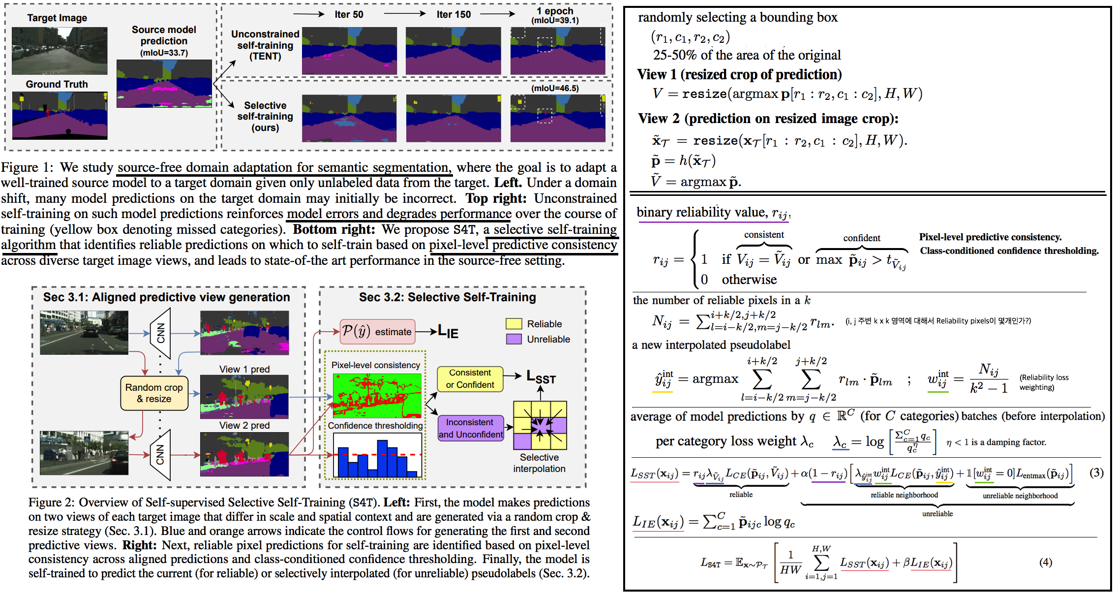
Abstract & Introduction

• Setting: Source free
• 제안 기법: Self-Supervised Selective Self-Training
  1. pixel-level predictive consistency (across diverse views of each target image) (along with model confidence) -> pixel predictions이 reliable인지 아닌지 판단한다.
  2. self-training with pseudo labels (for reliable predictions) or (via a selective interpolation strategy for unreliable predictions)
• TENT 문제점 (Unconstrained self-training) :
  1. Entropy Error에 의한, Error accumulation
  2. (Figure 1: Entropy Loss를 사용하면 Dominant class prediction & Unstable soft pseudo label 문제가 발생하는 것을 눈으로 직접 확인이 가능하다)

Method

• 그림과 같이 View1, View 2를 만든다. 그리고 Reliability signals만을 사용해 학습하는 Selective Self-Training을 수행한다.
• Pixel별 Binary Reliability Value를 측정하기 위해, 아래의 2 방법을 사용한다. (k=3 works best)
  1. Pixel-level predictive consistency
  2. Class-conditioned confidence thresholding: 하나의 고정된 Threshold만을 사용하는 것은 충분하지 않다. 왜냐하면, 카테고리 마다 output probability distributions이 다를 것이기 때문이다. 따라서 adaptive per-category confidence threshold를 사용할 것이다. batch 이미지들에 대한 probabilities를 추출하고, 각 클래스마다 threshold (t_c)보다 큰 confidence를 가지는 pixel이 50개 정도가 되도록 t_c를 설정한다.
• Loss Function
  1. Reliable pixel: Cross-entropy loss 사용
  2. Unreliable pixel: 중요한 pixel 정보로써 loss로 사용할지 아닐지를 먼저 정해야 한다. 아래의 2가지 방법을 사용한다.
     1. reliable neighborhood -> selective label interpolation을 사용해서 pseudo label를 찾는다. (+ reliability loss-weighting 적용, (w)
     2. unreliable neighborhood -> entropy maximizing (Probability를 평평하게 만든다. Entropy minimization이 TENT였다) (SENTRY 논문 참조)
• Selective self-training.
  • BN 파라미터만 update
  • imbalance across categories 문제를 해결하기 위해서, log-inverse frequency loss-weighting [63] 를 적용해서 Cross Entropy Loss를 가해준다. q를 batch 내부에서 예측된 Class 비율 vector라고 했을때, 수식이 그림과 같이 적용될 수 있다. (확실히는 모르겠고, 그냥 Focal Loss처럼 많은 비율을 차지하고 있는 class에 대해서 weight가 약하게 작동하는 거라고 생가하자) (λ)
  • information entropy loss(Loss . Trin / _IE): label imbalance문제를 해결하기 위해서, 모델이 다양한 클래스를 예측하도록 유도한다. Batch내부의 predictions q들을 모두 average하고 empirical prediction(지금까지 모아온 값)과 running average를 사용해서 Total prediction average q를 구한다. 이 q를 이용해서 entropy maximizaiton을 수행한다. (Entropy loss에 -를 제거한 값. average q가 평평하도록 유도한다. 자세하고 정확한 사항은 [59] 참조, 혹은 코드 참조 필요함)

6.2 Generalized Source-free DA -> Continual source-free DA

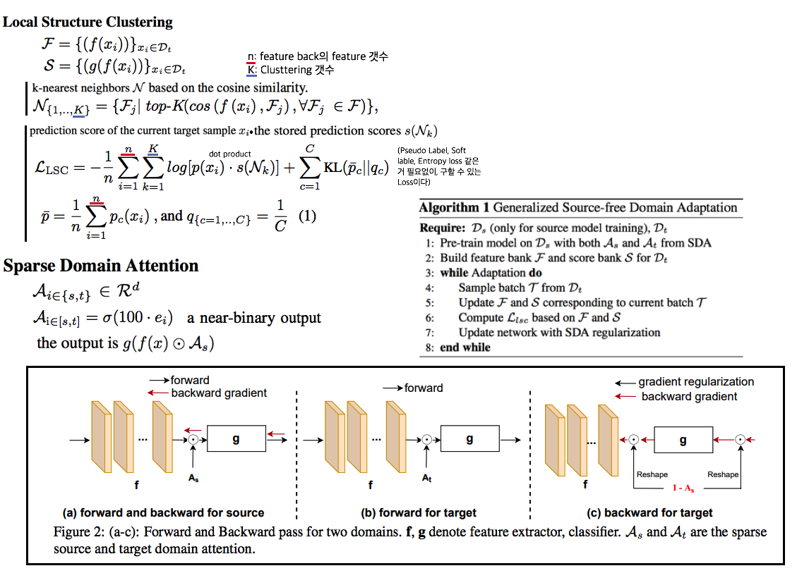
Abstract & Introduction

• 이전 Source free work들은, source의 성능 하락은 무시하고 target에서의 성능향상만을 고집했다. soure optimized model은 high practical value 이므로 source에서도 성능저하가 일어나지 않는 모델 개발을 목표로 한다.
• 제안방법1 local structure clustering (LSC) : Clustering the target features (with its semantically close neighbors) 함으로써 target domain에서 성능을 향상시킨다.
• 제안방법2 sparse domain attention (SDA) : a binary domain specific attention으로써 다음의 2가지 역할을 한다. 역할 (1) activate different feature channels for different domains 역할 (2) regularize the gradient to keep source information.
• continual source-free domains 으로의 확장을 이룬다.
• source domain에 접근하지 않고 학습을 하다보면 source의 성능저하가 일어난다. 4 계절이 존재하는 나라에서 그 계절은 주기적으로 바뀌기 때문에, 이런 상황은 옳지 못하다.

Methods

• Local Structure Clustering
  • Main Idae: Domain shift된 target domain feature가 생성될지라도 feature들은 class에 맞춰 cluster되어 있을 것이다. 그리고 nearest neighbors of target features는 같은 category labels을 공유할 가능성이 크다는 가정하에 Moving clusters of data points를 목표로 하여 LSC를 수행한다.
  • Loss를 적용하는 과정은 다음과 같다.
    1. Target domain feature bank를 모은 후, k-nearest neighbors (cosine similarity)를 적용한다.
    2. LSC loss를 적용하여, Feature가 cluster되도록 유도한다.
    3. Loss의 첫번쨰 텀은 Current target sample의 Feature자체가 자신의 Neighbors에 근처에 위치되도록 유도한다.
    4. Loss의 두번째 텀은 모든 Class에 대해서 balance한 예측을 하도록 유도한다.
    5. Current target sample (x)는 LSC 를 계산하는데 사용된 후, Bank stack에 저장된다.
• Sparse Domain Attention
  • continual learning methods을 적극적으로 활용한다.
  • Source 학습에 추가과정이 필요하다. Binary Attention (As)도 학습되어야 한다. (Attention은 Feature masking이라고 표현할 수 있다.)
  • Target에 의한 학습으로 source의 forgetting이 일어나지 않도록, 1 - Binary Attention (As) 이 적용하여 target에 의한 loss backpropagation이 이뤄지도록 유도한다.
  • 이러한 Layer는 Backbone의 가장 마지막 layer와 classifier의 가장 마지막 layer. 총 2개의 layer에만 적용한다.

6.3 SENTRY: Selective Entropy Optimization via Committee Consistency for Unsupervised Domain Adaptation

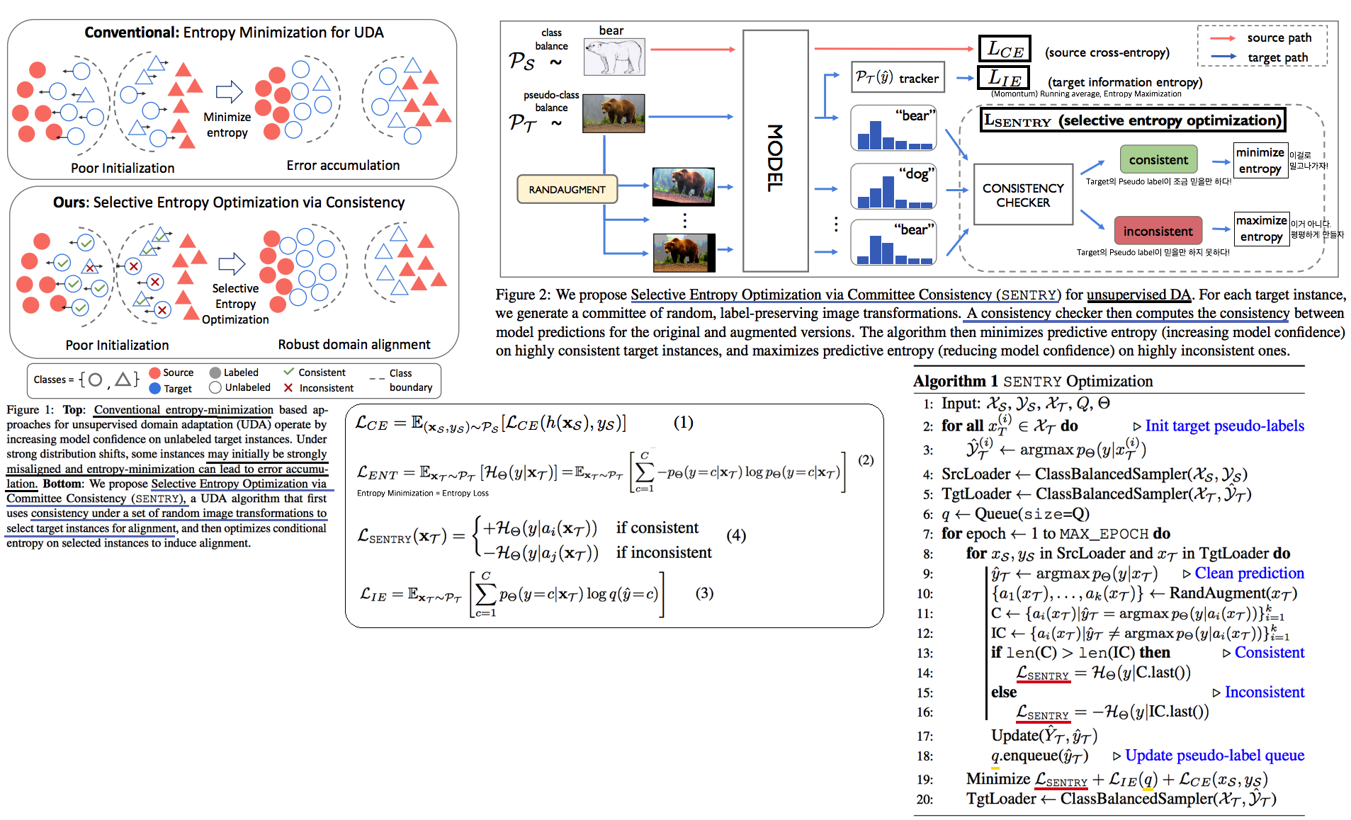
Abstract & Introduction

• Domain shift가 일어나면, label distribution shift 또한 일어난다. 따라서 prediction score의 변화가 일어나는 것은 당연하다.
• 기존 UDA들인 매우 불안정하다. [noisy pseudo-labels or entropy minimization over potentially miscalibrated predictions] 때문에.
• 따라서 constrained self-training 이 필요하다.

Method

• Entropy Loss 의 문제점 (1) Error accumulation (2) Prediction the majority class (dominant class prediction)
• information entropy loss(L_IE) 를 사용해서 문제를 해결한다. (#6.1의 [59] == #6.3의 [21] 이 논문을 참조해서 만든 Loss이다. 하지만 #6.3에서는 Running average를 사용하지 않는다. Classificaion에서는 이미 batch를 크게 해서 그런지 모르겠다. 그리고 논문, 코드(Line 78~Line101. Line93,94가 핵심)를 봐도 이해가 힘들다. 필요하면 좀 더 공부가 필요하다.)
• SENTRY는 다음과 같다. Target Image를 여러번 Transform해보고, 다중 예측을 해봐서 같은 예측이 많이 나오면 Target Pseudo label이 믿을만 한거다(case A). 그렇지 않으면 Target Pseudo Label이 믿을만 하지 않은거다(case B). 만약 Case A라면, 그것을 확실히 믿고 Entropy Loss를 적용한다. 만약 Case B라면, 그것은 믿을 만하지 않으므로, Prediction을 다시 해보게끔 scour를 평평하게 만들어주는 Entropy Maximization을 적용해준다.

6.4 Adapting ImageNet-scale models to complex distribution shifts with self-learning

Abstract & Project Page

• Self-learning을 robustness관점에서 ImageNet을 활용한 종합적 평가를 수행했다.
• Self 기법으로는 Robust pseudo-labeling(RPL), entropy-minimization 를 활용했다.
• 그들이 찾은 핵심 2가지는 다음과 같다
  1. short updat를 사용해야한다. (Table6. 작은 iter가 아니라 계속 teacher=student 로 사용해야한다는 것을 의미한다.)
  2. few BN parametor만 학습하는게 좋다 (Table7)
  3. label noise에 대응하기 위해서는, Robust Pseudo-Labeling 기법을 활용해야한다. (Table2)
• 이러한 핵심을 바탕으로 ImageNet-C,R,A (Corruptions due to JPEG artefacts, noisy. ImageNet-C) 에서 SOTA

Self-learning for Domain Adaptation

• 다음의 UDA 기본학습과정을 따른다. f0 → f1 → f2 … teacher & student model 관점으로 학습을 진행한다. teacher model 에서 나온 예측 결과 중 일정 Threshold가 넘는 data에 대해서 student를 학습시키는데 사용한다. teacher predictions를 어떻게 사용할지는 다음의 3가지 기법 중 하나를 따른다. 그리고 이 논문은 RPL이라는 기법을 새로 제시한다.
  1. Hard Pseudo-Labeling: teacher model hard predictions을 GT로 사용
  2. Soft Pseudo-Labeling: teacher model soft predictions을 GT로 사용
  3. Entropy Minimization: student model soft predictions을 GT로 사용
  4. Robust Pseudo-Labeling (RPL)
     • 위의 기법들의 Cross Entropy 수식은 label noise에 sensitive 하다.
     • teacher predictions 사용하는 것은 부적절하다. (Table6참조) student label 사용해야 한다.
     • label noise에 강인한 Generalized Cross Entropy (GCE) 를 사용한다. 이것은 Mean Absolute Error (MAE) loss [16] 와 Cross entropy loss와의 결합이다.
     • GCE with hard-labeling을 사용하고 short update intervals 학습으로 가장 좋은 성능을 낼 수 있었다.

Experiment design

• Hyperparameters: We consider three choices: (i) the parameters of the last network layer, (ii) the affine batch normalization parameters or (iii) all trainable parameters. SGD optimizer.

6.@ Compositional Models: Multi-Task Learning and Knowledge Transfer with Modular Networks

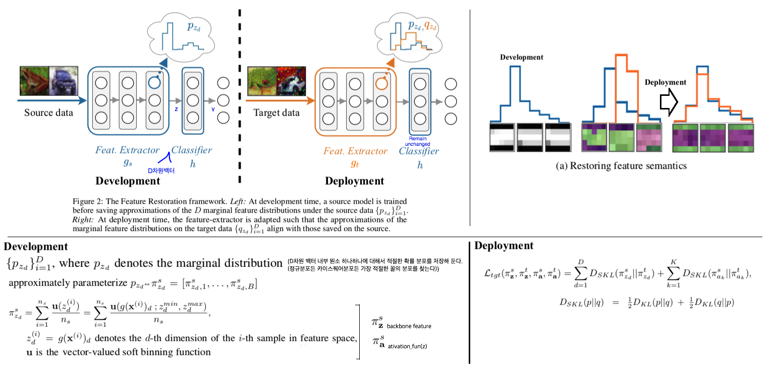
6.5 Source-Free Adaptation to Measurement Shift via Bottom-Up Feature Restoration

Abstract

• source학습과정 중, feature distribution를 저장한다. target이 들어올 때, feature distribution을 source의 것과 비슷하게 맞춘다. 이 것을 Feature Restoration이라고 표현한다. 더 나아가, Bottom-up Feature Restoration을 제안하다.

Setting

• Development time: Feature distribution (statistics)를 저장한다.
  • Step1: 가장 적절한 feature distribution 선택하기. D차원 백터를 모두 다 저장하는 것은 옳지 않으므로, “histograms를 분석하는 soft binning function이라는 기법을 사용해서, only the marginal feature distributions”만을 저장한다.
• Deployment time
  • 주어진 것은 다음의 3개이다. (1) pre-trained source model (2) lightweight statistics (3) unlabelled target examples
  • Feature store을 수행한다. target distribution이 위에서 저장된 source distribution과 동일하도록 유도한다.
  • Feature extractor(g_t) 에만 Loss를 걸어주고, Classifier는 그대로 고정한다.
  • Bottom-Up Feature Restoration: 초기 layer 먼저 source distribution과 비슷한 feature가 나오게 유도해준다면 target의 특별한 brightness or blurring등에 잘 적응하는 모델이 될 것이다. 이러한 직관을 따라서 bottom-up방식으로 training은 block layer부터 몇 epoch씩 학습시켜주는 방식을 사용했다. (30 epochs per block)

6.6 Source-Free Open Compound Domain Adaptation in Semantic Segmentation

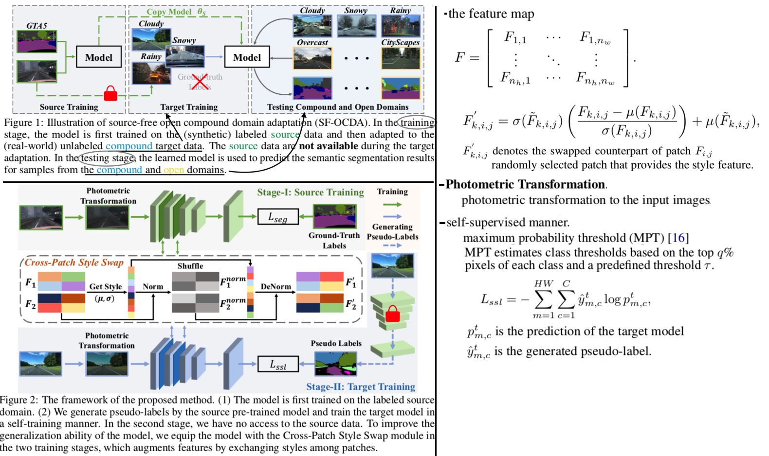
Abstract & Instruction

• 더 Practical한 Source Free => Data privatcy and data storage Issue / Compound 이상의 unseen open target domain에 대한 적응
• 2가지 Step을 제시한다. (1) Cross-Patch Style Swap(SPSS) (2) Adapting with self-learning
• CPSS: features with various patch styles를 augmentation한다. → the generalization ability of the model → 정확한 pseudo-labels 생성 가능

6.7 OVANet: One-vs-All Network for Universal Domain Adaptation

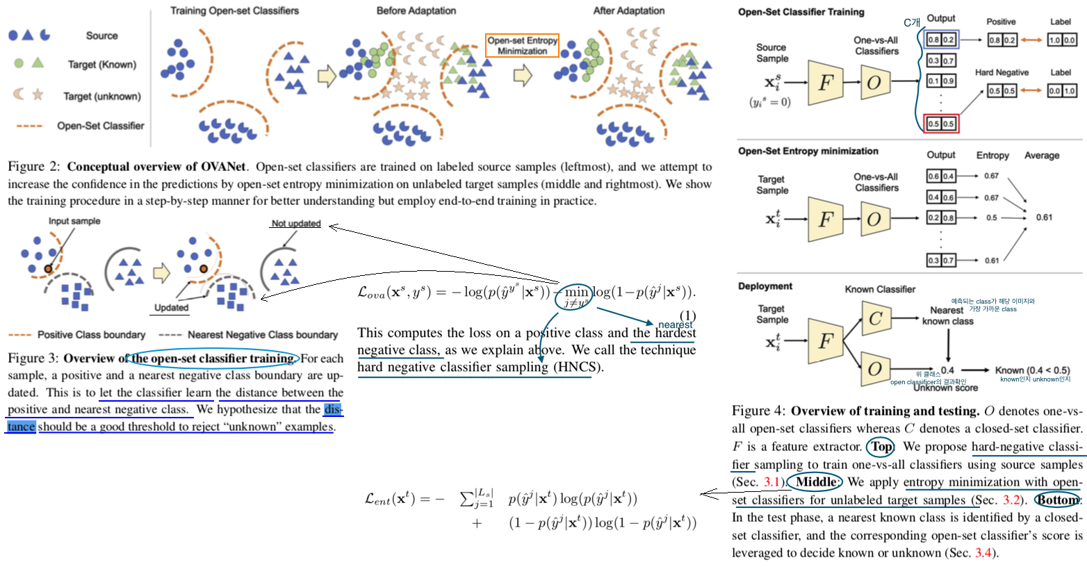
• Universal Domain Adaptation (UNDA) : domain-shift and category-shift (Unknown class 까지 분별하는 능력을 갖춘 모델)
• 지금까지 Method는 Manual threshold를 사용하지만, 이 논문에서는 certainty를 learnable하게 예측하는 Network를 사용한다. 이 Network를 Open set classifier라고 부르고, class를 예측하는 것은 closed set claasifer라고 부른다. 핵심적으로 Open set classifier는 Class 갯수 만큼 존재하며, Output으로 2차원 백터가 나온다. 이 백터는 unknown인지 known인지를 판단해준다.
• 그리고 Entropy minimization을 closed set claasifer에 적용하는게 아니라, Open set classifier에 적용함으로써 Target Adaptation을 수행힌다.

6.7 Domain-Specific Batch Normalization for Unsupervised Domain Adaptation -CVPR2019

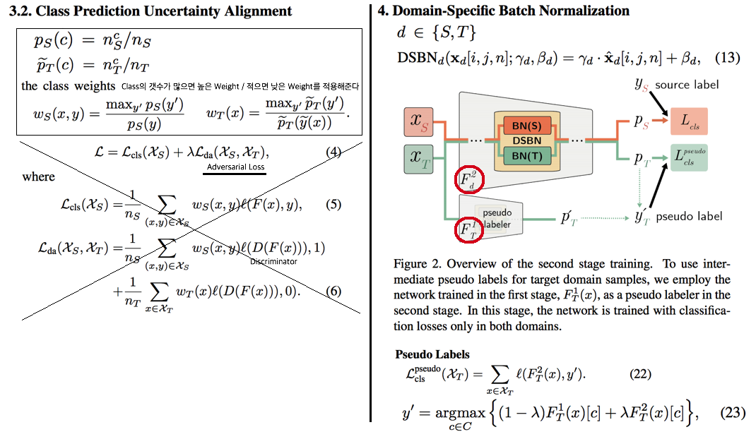
1. Train pseudo labeler. (CPUA,2018)
   • CPUA[14, 왼쪽 수식]을 사용해서 F1_T를 학습시킨다. Adversarial Learning에 의해서 BN(T), F1_T 가 Update된다.
2. Self-training with Pseudo Labels.
   • Target Pseudo Label[오른쪽 아래 수식 참고]을 생성해서 F2_T를 학습시킨다.
3. 이렇게 학습된 모델 중, 일반적으로 F2_T가 F1_T 보다 정확하다고 한다. 두번째 Stage에 의해서 F2_T가 좀더 정제되고 정확한 Pseudo Label에 의해서 학습되기 때문이다. 따라서 Equ23. λ를 점차 증가하면서 Pseudo Label을 만들어 낸다.
4. DSBN 코드는 아래와 같다
   • DSBN Model : https://github.com/wgchang/DSBN/blob/master/model/dsbn.py (주의, 여기서 num_classes 는 Reference될 때, self.num_domains 가 들어간다. 헷갈리지 말 것.)
   • Resnet_dsbn : https://github.com/wgchang/DSBN/blob/master/model/resnetdsbn.py

6.8 Learning to Optimize Domain Specific Normalization for Domain Generalization

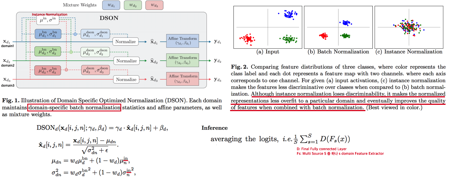
• Incorporating optimized normalization layers that are specific to individual domains
• By linearly interpolating the means and variances of the two normalization statistics → batch and instance normalizations의 적절한 조합
• Inference하는 동안 Target Domain가 들어온다. 모든 Domain의 Feature Extractor를 사용해서 Logits (softmax 이전) 을 계산하고 그것을 Averageing하는 방식으로 Target Prediction을 예측한다.

6.9 Batch Normalization Embeddings for Deep Domain Generalization

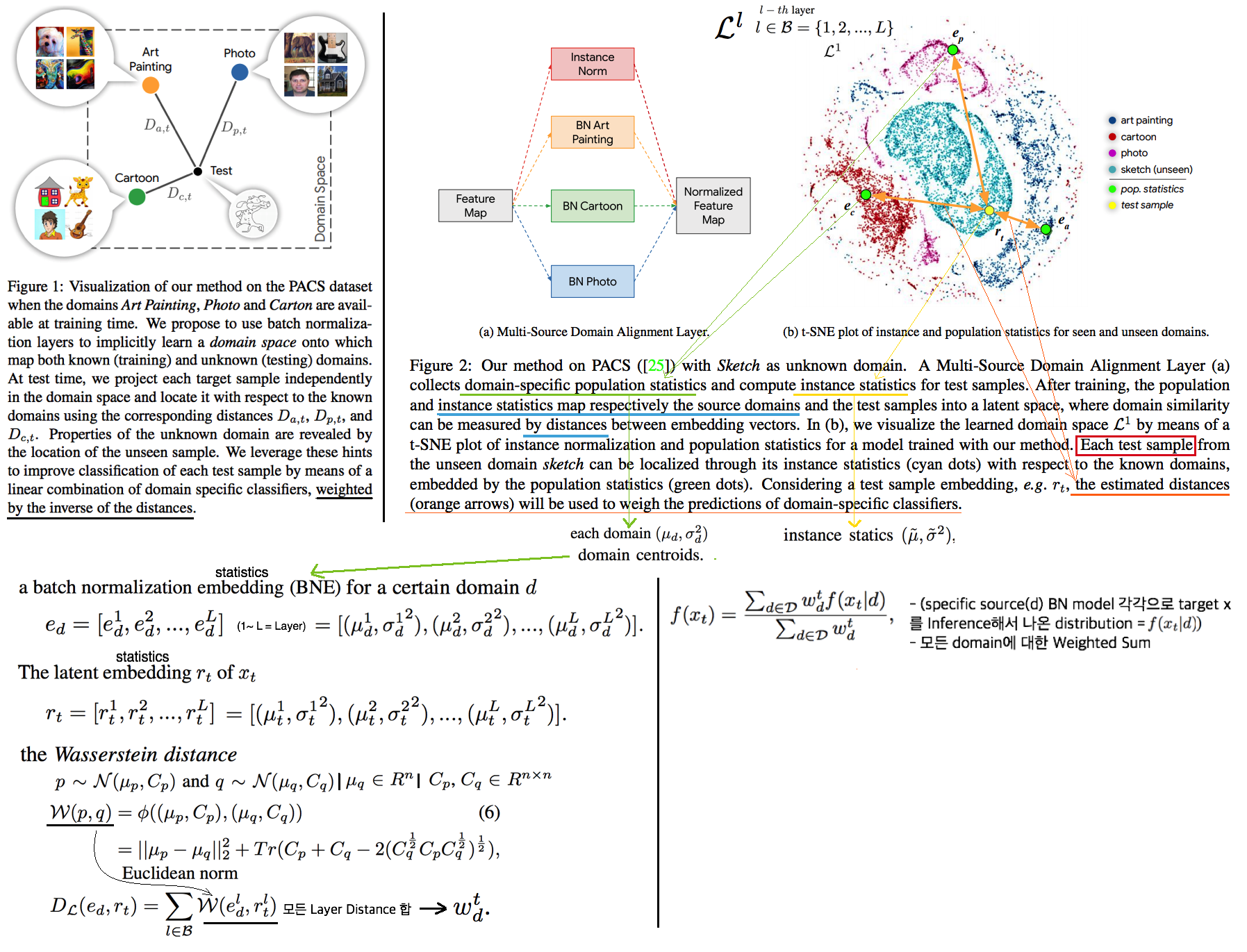
1. we explicitly train domain-dependant representations by using domain-specific batch normalization layers to collect independent domain’s statistics.
2. At test time, we project unkown samples into the same space as a linear combination of the known ones. the weights depends on the similarity of a test sample to each source domain will be used. (weighted sum)
3. 이를 통해서 Learning a powerful but lightweight ensemble model 얻을 수 있다.
4. 위 이미지 설명
   • e 는 domain centroid statics이다. (사실상 e는 BN layer의 running_mean / running_std 일 것 이다)
   • r 는 새로 들어온 target에 대한 Feature statics이다. 모든 layer(1 ~ L)에 대한 statics를 모으면 다음과 같은 집합으로 표현할 수 있다.
   • e와 r을 wasserstein distance를 사용해서 두 Domain 사이의 Distance를 예측한다.(C와 σ와의 관계는 공부가 필요하다) 수학적 수식은 위와 같다. Weight(distance)는 하나의 float값이 나와야 하기 때문에 모든 Layer에 대한 distance를 Average sum하는 방식으로 Weight(distance)를 계산한다.
   • Weight(distance) 를 사용해서 Target prediction score를 계산한다. 모든 Source BN model에 Forward를 해야 한다는 cost가 발생한다.
5. Two distribution comparison / two multivariate gaussians / normal distiributions
   1. KL divergence without covariance [Marg. Gauss]
   2. KL divergence with covariance [stackexchange]
   3. Wasserstein distance [위 수식 참조]
   4. Bhattacharyya [wiki]

6.7 Federated Multi-Target Domain Adaptation

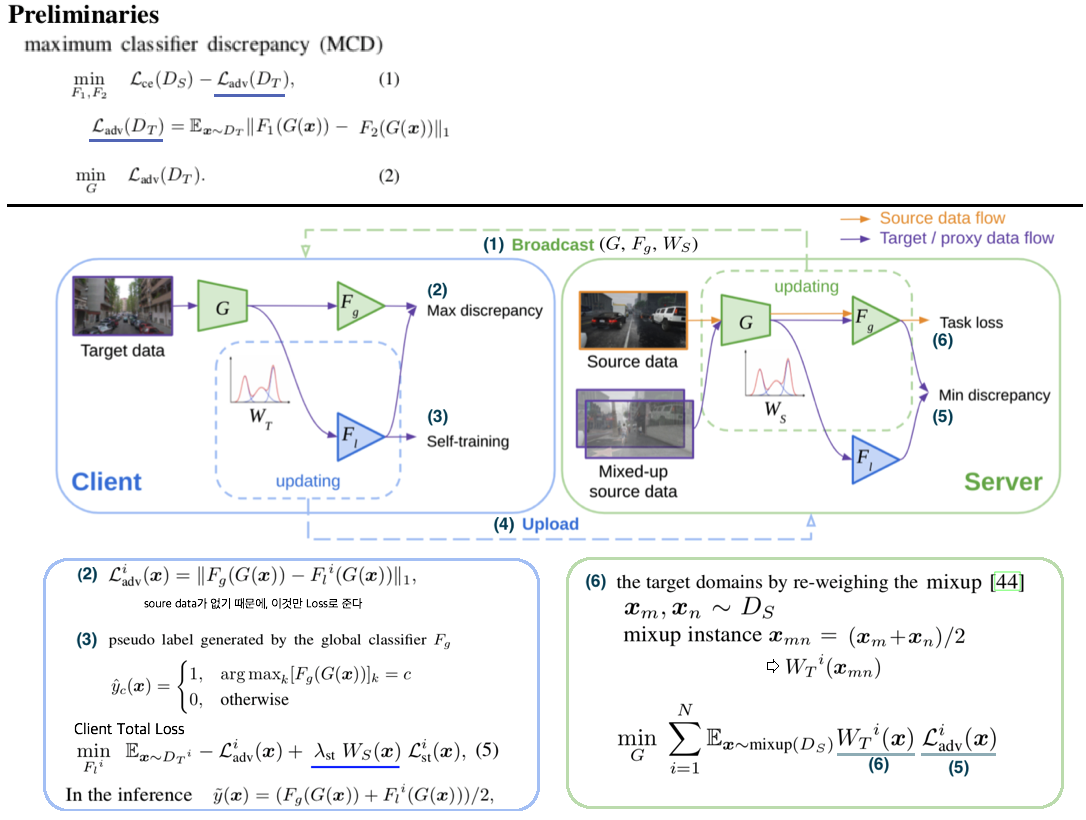
Abstract & Instruction

1. Federated Learning이란 client data의 privacy를 보호하면서, distributed model을 학습하고, 최종적으로 General central model 을 획득을 목표로 한다.
2. 따라서 사용할 수 있는 데이터는 2가지 이다. (1) unlabeld Client data (2) labeled centralized data
3. 이런 세팅에서의 Challenge는 다음과 같다. (1) Multi client target (2) Unlabeled target (3) target domain shift
4. Multi party learning framework가 필요하다. 모든 participants의 데이터는 보호해 주면서, 모델 파라미터만! 서로 interact 가능하다.

Method

1. MCD (maximum classifier discrepancy): 그림의 Equ(1) 을 의미한다. Equ(1)의 좌항은 source label과의 cross entropy loss를 말하고, 우항은 각 Classifier F1,F2가 항상 서로 다른 결과가 나오도록 강제하는 수식이다. 반대로 Equ(2)를 통해서 F1,F2 무엇을 통과하든 같은 결과가 나오도록 강제하는 수식이다.
2. Client Total Loss에서 W_s는 source distribution을 말한다. domain shift로 Fg가 target에 적합하지 않을 수 있다. 따라서 target이 source와 비슷했을 때만 강한 self-sup-loss를 주는게 직관적으로 적절하다. (정확한 공식은 코드가 공개되지 않아서 알기 어려움. GMM model/parameter (Gaussian mixture model) 라는 말이 논문에 많이 나오는데 지금은 이게 뭔지 모르겠고, 나중에 코드 레벨로 공부해보자)

6.8 Boosting Domain Adaptation by Discovering Latent Domains

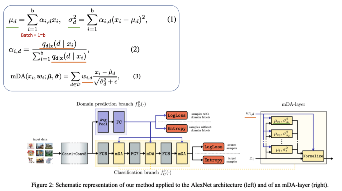
Abstract

1. In practive, (1) Source는 Mixtures of multiple domains (2) Source의 domain label이 없을 수도 있다.
2. 따라서 (1) Domain Classifier로 latent domain을 감지하고. (2) novel layer에서 그 domain 정보를 사용하는 방법을 제안한다,

Method

1. Labeled source dataset / unlabeled target dataset / partialy domain label 이 존재한다. domain label은 k+1개로 한다. k는 source를 분류한 갯수이고 (순전하 하이퍼파라미터이다) 1은 target domain을 의미한다.
2. Multi-domain DA layers
   1. domain shift를 줄일 수 있는 방법으로, domain specific하게 normalization하는 방법이 있다.
   2. 이때 Norm을 위한 m_d, std_d (d=특정 domain d) 를 계산할 필요가 있다. 이를 계산하기 위해서 Equ(1), Equ(2)를 사용한다.
   3. Equ(2)에서 q_d는 x_i 이미지가 domain일 확률을 의미한다. 만약 domain label이 있다면 q를 정의하는 건 쉽지만 q가 없다면 domain prediction network를 사용한다.
   4. 이렇게 구한 q를 이용해서 alpha를 계산하고 mean, std를 Equ(1)와 같이 계산한다.
   5. 그리고 q는 w_id로 대체되어 또 다시 사용된다. w는 해당 domain normalizaiton을 얼마의 weight로 사용할건지를 의미한다.
3. Domain prediction Network
   1. 이 Network에서 나오는 k개의 확률값은 q와 w로 사용된다. 하지만 source의 domain label이 존재하거나 target 이미지가 들어온다면 prediction probability 를 사용하지 않는다. 이미 알고 있는 domain 정보를 그대로 사용한다. (mDA layer에도 mean_t, std_t 가 존재한다.)
   2. 너무 깊은 layer feature를 해당 network의 input으로 사용하면 feature의 domain invariant가 커져 network가 잘 학습되지 못한다. 따라서 적절한 깊이의 feature를 input으로 하여 predictor 가 domain probability를 예측한다.
4. Training the network
   1. 논문에서는 복잡하게 쓰여있다. 위 Network 그림을 봐도 어떤 Loss를 사용했는지 알 수 있다. label이 있으면 cross entropy loss를 사용했고, label이 없으면 entropy loss를 사용했다. (label에 매우 의존적인 network가 될테지만.. 이 논문에서는 그냥 이렇게 사용했다.)

6.9 Generalize then Adapt: Source-Free Domain Adaptive Semantic Segmentation

Abstract

1. a virtually extended (가상으로 만들어진) multi-source dataset 을 사용해서 source only gerneralization을 이룬다.
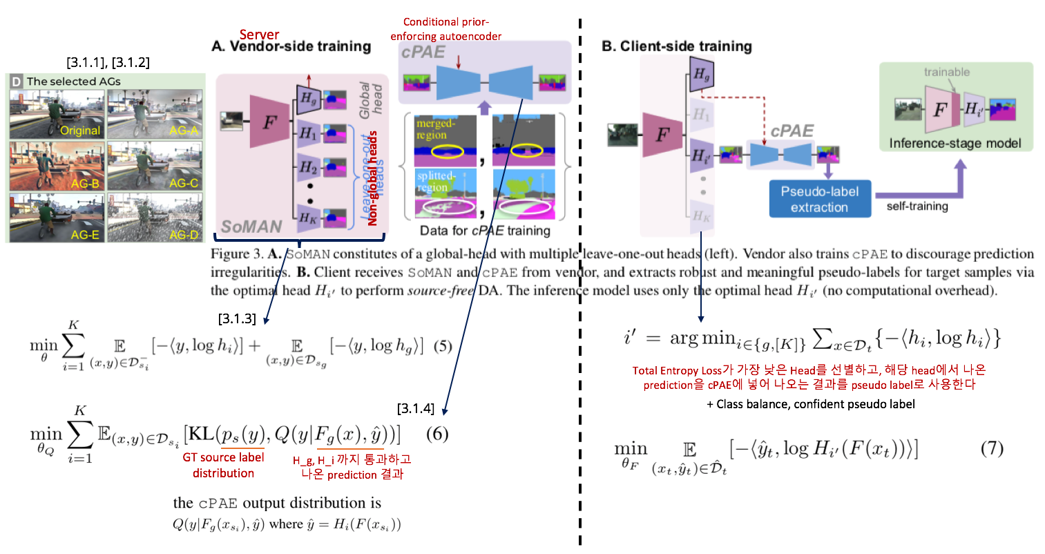
2. reliable target pseudo label을 추출하여 target adaptation을 수행한다. pseudo-label quality를 향상시키기 위해서 “conditional prior-enforcing auto-encoder“라는 새로운 method를 사용했다.

Method

1. [3.1.1], [3.1.2] 내용은 domain-varying augmentation을 한 방법을 소개한다. 필요하면 찾아 읽어 볼 것.
2. [3.1.3] Source-only Multi-Augmentation Network == classifier가 multi head로 존재하는 network 이다. classifier의 개수는 총 1+K개이며, 여기서 1은 global, K는 augmented style dataset의 갯수를 의미한다. global classifier는 모든 dataset을 가지고 학습되며, non-global head K개는 각 style dataset만을 가지고 학습된다. 이를 수식으로 표현하면 Equ(5) 와 같이 표현할 수 있다.
3. [3.1.4] irregularities (“car flying in the sky”, “grass on road”, “split car shape”, “merged pedestrians”) 를 해소할 방법으로 Prior-enforcing Auto-Encoder (cPAE)를 제안한다. denosing auto-encoder network 라고도 표현할 수 있다. 이것 학습시키는 Loss는 Equ(6) 와 같다.
4. [3.2.1] Total Entropy Loss가 가장 낮은 Head를 선별하고, 해당 head에서 나온 prediction을 cPAE에 넣어 나오는 결과를 pseudo label로 사용한다. 또한 Class balance, confident pseudo label을 만들기 위해서 각 class마다 Top 33% confidence를 threshold로 사용하고 33% 이내의 confidence를 가지는 class-prediction-result만 Pseudo label로 사용한다.