【IE】 Zero-Reference or Low-Light Image Enhancement
- Paper: Zero-Reference Deep Curve Estimation for Low-Light Image Enhancement
- Type: Image Enhancement
- Reference site:
- Contents
Zero-Reference or Low-Light Image Enhancement
1. Abstract, Introduction, Relative work
- Zero-Reference: Paired or Unpaired Dataset이 필요 없음
- Deep Curve Estimation: Pixel value Function을 정의하는 함수의 파라미터를 예측.
- non-reference loss functions: 4가지 종류의 Loss로 이뤄져있으며, Self-Supervision이다.
- 추가적 장점, the potential benefits to face detection in the dark.
- 전통 기법
- Retinex theory [13]: reflectance and illumination 부분을 추정하는 이론.
- uan and Sun [36]: 주어진 이미지에서 ` global optimization algorithm` S-shaped curve를 추정하고 그대로 이미지에 적용
- 딥러닝 사용 기법
- CNN based
- Pared data 필요
- Wang et al. [28, 2019 CVPR]: estimating the illumination map. paired data that were retouched by three experts.
- GAN based
- Unpared data 사용
- EnlightenGAN [12, 2019 CVPR]: unpaired low/normal light data와 GAN을 사용해서 low-light Image Enhancement. 그러나 careful selection of unpaired training data이 필요하다는 문제점 있음
- CNN based
- 지금까지의 다른 기법들 문제점
- Fail to cope with the extreme back light region
- Generate color artifacts
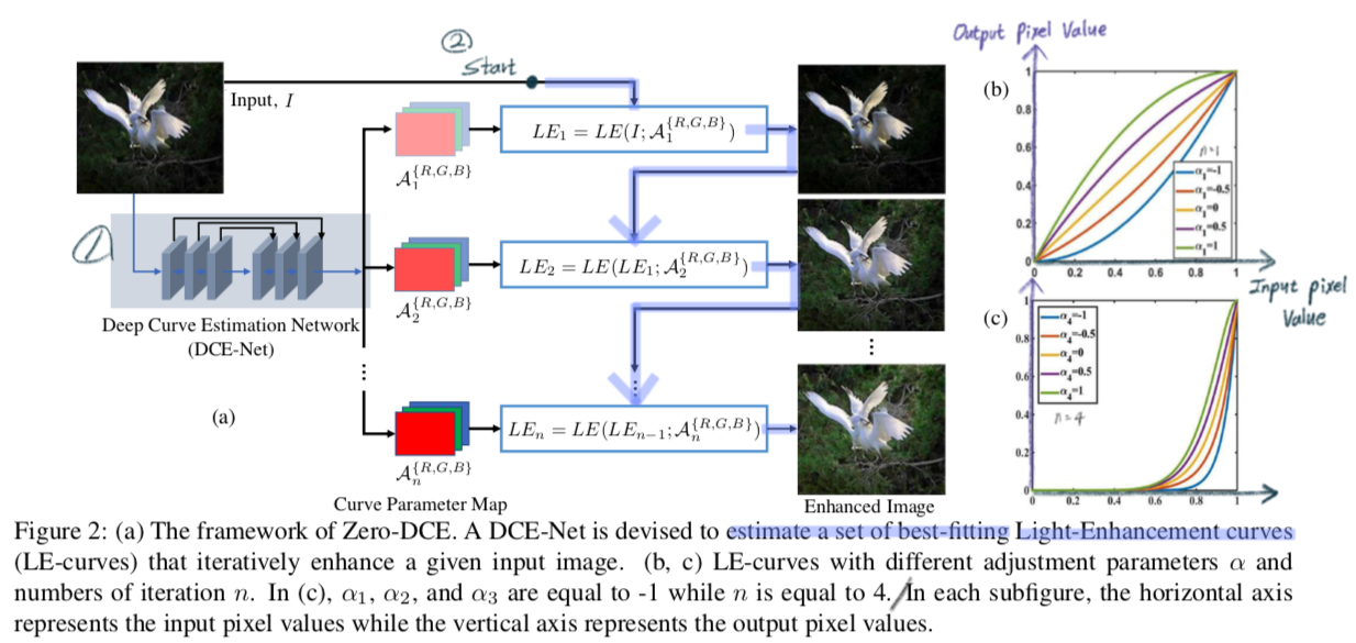
2. DCE-Net
- Input: Image (256×256×3)
- Output: a set of pixel-wise curve parameter maps for corresponding higher- order curves
- a plain CNN of seven convolutional layers with 32 convolutional kernels of size 3×3.
- ReLU activation function.
- down-sampling 그리고 batch normalization layers 는 없다.
- Last: Tanh activation function, 24 channels (8 iterations (n = 8) x RGB(3) )
- RGB 따로 추정하여 얻는 장점
- Better preserve the inherent color
- Reduce the risk of over-saturation
3. Light-Enhancement curves
Estimate a set of best-fitting Light-Enhancement curves by alpha, α [-1, 1] 사이의 값
Curve 조건
- each pixel value in the normalized range of [0,1]
- this curve should be monotonous. (단순 증가 함수, 단순 감소 함수)
- simple and differentiable

LE-curve의 장점
- E-curve enables us to increase or decrease the dynamic range of an input image
- Not only enhancing low-light regions But also removing over-exposure artifacts.
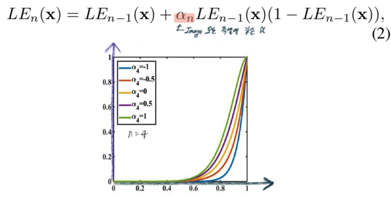
Higher-Order Curve
- The LE-curve defined in Eq. (1) can be applied iteratively.
- Global adjustment since α is used for all pixels. But a global mapping tends to over-/under- enhance local regions.
- n = 1~8
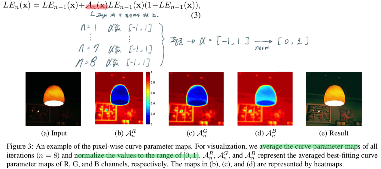
Pixel-Wise Curve
- 각각의 픽셀이 다른 alpha, α 값을 가질 수 있도록 공식 수정
4. Non-Reference Loss Functions
4.1. Spatial Consistency Loss
- Encourages to preserve spatial coherence
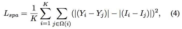
- K is the number of local region(이미지 4x4 Poolling) / Ω(i) is the four neighboring regions (top, down, left, right)
- Y and I as the average intensity value of the local region in the enhanced version and input image
- 코드
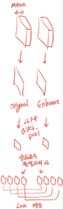
4.2. Exposure Control Loss
- the well-exposedness level E. We follow existing practices [23,24]. We set E to 0.6
- M represents the number of nonoverlapping local re- gions of size 16×16, Y is the average intensity value
- 코드
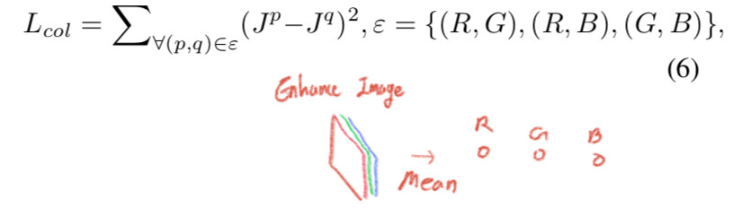
4.3. Color Constancy Loss
- “Color in each sensor channel averages to gray over the entire image” 이라는 가정 이용 [논문참조, 2]
- Encourage to correct the potential color deviations in the enhanced image.
- 아래 수식의 J_p denotes the average intensity value of p channel
- 코드
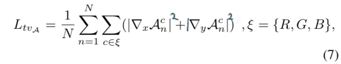
4.4. Illumination Smoothness Loss
- To preserve the monotonicity relations between neighboring pixels
- 코드
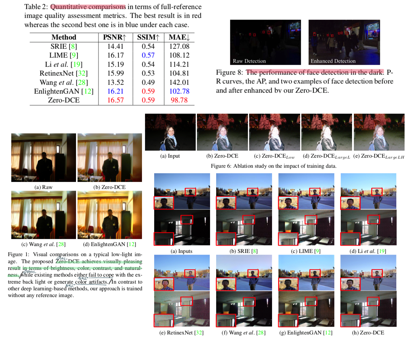
5. Results