【Se-Segmen】Rethinking Semantic Segmentation with Transformers
- 논문 : Rethinking Semantic Segmentation from a Sequence-to-Sequence Perspective with Transformers
- 분류 : Semantic Segmentation
- 저자 : Sixiao Zheng, Jiachen Lu, Hengshuang Zhao
- 느낀점
- 목차
- Paper Review
Rethinking Semantic Segmentation
1. Conclusion, Abstract
sequence-to-sequence prediction framework를 사용해서 Semantic Segmentation을 수행해 보았다.- 기존의 FCN들은
- Encoder, Decoder 구조를 차용한다. CNN을 통과하면서 resolution을 줄이고
abstract/semantic visual concept을 추출한다. - receptive field를 넓히기 위해서
dilated convolutions and attention modules를 사용했다.
- Encoder, Decoder 구조를 차용한다. CNN을 통과하면서 resolution을 줄이고
- 하지만 우리는 global context 를 학습하기 위해 (= receptive field를 넓히기 위해서)
every stage of feature learning에서 Transformer 를 사용했다.pure transformer (without convolution and resolution reduction) - (Panoptic deeplab 처럼) 엄청나게 복잡한 구조를 사용하지 않고,
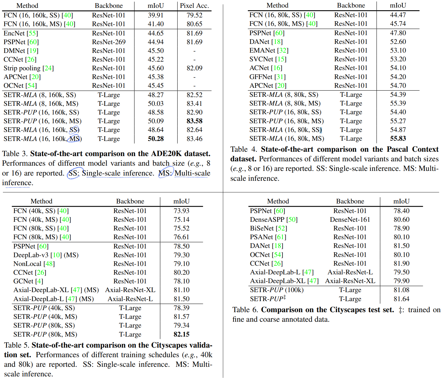
decoder designs을 사용해서 강력한 segmentation models = SEgmentation TRansformer (SETR) 을 만들었다. - Dataset에 따른 결과 : ADE20K (50.28% mIoU), Pascal Context (55.83% mIoU), ADE20K test server(1 st, 44.42% mIoU)
3. Method
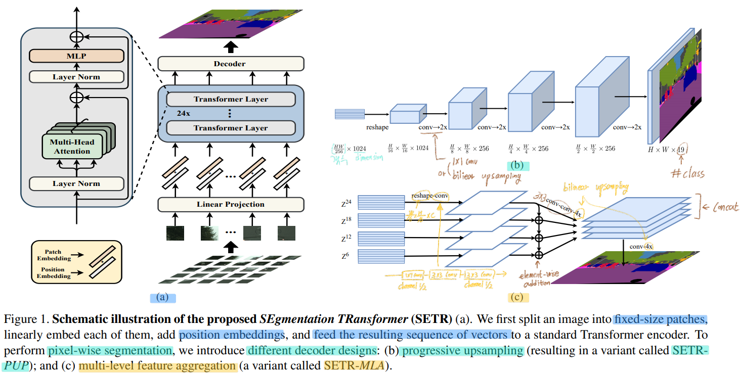
- 위의 이미지는 아래의 것에 대한 이미지 이다.
- (맨왼쪽) Transformer layer
- Image (transformer) Encoder
- (오른쪽 위) 두번째 Decoder : SETR-PUP
- (오른쪽 아래) 세번째 Decoder : SETR-MLA
- 첫번쨰 Decoder인 Naive에 대한 이미지는 없다.
3.1. FCN-based semantic segmentation
- About receptive field
- typically 3×3 conv를 사용하는 layer를 deep하게 쌓으면서 linearly하게 receptive field를 증가시킨다.
- 결과적으로, 높은 layer에서 더 큰 receptive fields를 가지게 되서 layer depth dependency가 생기게 된다.
- 하지만 layer를 증가시킴으로써 얻는 benefits에는 한계가 있고, 특히 특정 layer이상으로 가면 그 benefits가 빠르게 감소하는 형상을 볼 수 있다.
- 따라서, 제한적인
receptive fields (for context modeling)가 FCN의 본질적인 한계라고 할 수 있다.
- Combination of FCN with attention mechanism
- 하지만 이런 attention mechanism는
quadratic complexity때문에higher layers with smaller input sizes를 가져야한다는 한계점이 존재한다. - 이로 인해, 전체 모델은
lower-level feature만이 가지고 있는 정보들을 learning하지 못하게 된다. - 이러한 한계점을 극복하게 위해서, 우리의 모델은
pure self-attention based encoder를 전적으로 사용하였다.
- 하지만 이런 attention mechanism는
3.2. Segmentation transformers (SETR)
- Image to sequence
image sequentialization: flatten the image pixel -> 총 1D vector with size of 3HW 가 만들어진다.- 하지만 a typical image가 480(H) × 480(W) × 3 = 691,200 차원의 1차원 백터이다. 이것은 너무 high-dimensional vector이므로 handle하기가 쉽지 않다. 따라서 transformer layer에 들어가기 전에, tokenizing (to every single pixel) 할 필요가 있다.
- FCN에서는 H×W×3 이미지를 FCN encoder에 통과시켜서, H/16 × W/16 ×C 의 feature map을 뽑아 낸다. 이와 같은 관점으로 우리도 transformer input으로는 H/16 × W/16 (백터 갯수) x C(백터 차원) 으로 사용하기로 했다.
- 우리는 FCN의 encoder를 사용하는게 아니라
fully connected layer (linear projection function)을 사용해서 tokenizing을 한다. - 이미지를 가로 16등분, 세로 16등분을 해서 총 256개의 이미지 patchs를 얻어낸다. 그리고 이것을 flatten하면, HW/256 (백터 갯수) x C*(백터 차원) 를 얻을 수 있고, 이것을
linear projection function를 사용해서 HW/256 (=L: 백터 갯수) x C(백터 차원 < C*) 의patch embeddings결과를 뽑아 낸다. positional embeding: specific embedding p_i를 학습한다. i는 1~L개가 존재하고 차원은 C이다. 따라서 Transformer layer에 들어가기 전final sequence input E= {e1 + p1, e2 + p2, · · · , eL + pL} 가 된다. 여기서 e는patch embeding 결과그리고 p는positional emdeing값이다.
- Transformer
- a pure transformer based encoder
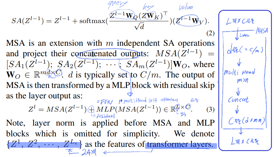
- 여기서 말하는 transformer layer는 위 이미지 가장 왼쪽의 Block 하나를 의미한다. 이것을 24개 쓴다.
- 즉 Transformer layer를 통과하고 나온 output 하나하나가 Z_m 이다.
- a pure transformer based encoder
3.3. Decoder designs
- three different decoder를 사용했다. 1.
Naive upsampling (Naive)2.Progressive UPsampling (PUP)3.Multi-Level feature Aggregation (MLA) - 이 decoder의 목표는 pixel-level segmentation을 수행하는 것이다. Decoder에 들어가기 전에, HW/256(갯수) × C(차원) 의 feature를 H/16 × W/16 ×C로 reshape하는 과정은 필수적이다.
- ` Naive upsampling (Naive)`
- simple 2-layer network (1 × 1 conv + sync batch norm (w/ ReLU) + 1 × 1 conv )를 사용해서 #class의 수를 가지는 channel로 만든다.
- 그리고 간단하게
bilinearly upsample을 사용하여 가로세로 16배를 하여 full image resolution을 만들어 낸다. - 그리고
pixel-wise cross-entropy loss를 사용해서 pixel-level classification을 수행한다.
Progressive UPsampling (PUP)- 쵀대한 adversarial effect (어떤 작업을 해서 생기는 역효과) 를 방지하기 위해서, 한방에 16배를 하지 않는다.
- 2배 upsampling 하는 작업을 4번을 수행한다.
- 이 작업에 대한 그림은
Figure 1(b)에 있고, progressive(순차적인, 진보적인) upsampling 으로써 SETR-PUP 이라고 명명했다.
Multi-Level feature Aggregation (MLA)- feature pyramid network와 비슷한 정신으로 적용하였다.
- 물론
pyramid shape resolution을 가지는 것이 아니라, FPN와는 다르게every SETR’s encoder transformer layer는 같은 resolution을 공유한다. Figure 1(c)와 같이, {Z_m} (m ∈ { L_e/M , 2*L_e/M , · · · , M*L_e/M }) 를 사용한다. 이미지에 나와있는 것과 같이, 다음의 과정을 수행한다. (1)reshape(2) ` top-down aggregation via element-wise addition(3)channel-wise concatenation`
4. Experiments
- Dataset : Cityscapes, ADE20K, PASCAL Context
- Implementation details
- public code-base
mmsegmentation[40], - data augmentation : random resize with ratio between 0.5 and 2, random cropping, random horizontal flipping
- training schedule : iteration to 160,000 and 80,000, batch size 8 and 16
polynomial learning rate decay schedule[60, 이건뭔지 모르겠으니 필요하면 논문 참조], SGD as the optimizer- Momentum and weight decay are set to 0.9 and 0
- learning rate 0.001 on ADE20K, and 0.01 on Cityscapes
- public code-base
- Auxiliary loss
- auxiliary losses at different Transformer layers
- SETRNaive (Z_10, Z_15, Z_20)
- SETR-PUP (Z_10, Z_15, Z_20, Z_24)
- SETR-MLA (Z_6 , Z_12, Z_18, Z_24)
- 이렇게 각 layer에서 나오는output을 새로 만든 decoder에 넣고 나오는 결과와 GT를 비교해서 Auxiliary loss의 backpropagation를 수행한다.
- 당연히 이후의 각 dataset 당 사용하는
Evaluation metric을 사용해서main loss heads에 대한 학습도 수행한다.
- Baselines for fair comparison
- dilated FCN [37] and Semantic FPN [28]
- Multi-scale test
the default settings of mmsegmentation[40] 를 사용했다.- 일단, uniform size 의 input Image를 사용한다.
- scaling factor (0.5, 0.75, 1.0, 1.25, 1.5, 1.75)를 이용하여, Multi-scale scaling and random horizontal flip 을 수행한다.
- 그리고 test를 위해서
Sliding window를 사용했다고 하는데, 이게 뭔소리인지 모르겠다. (?)
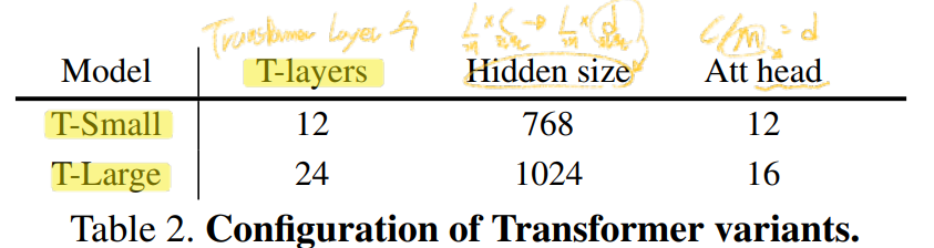
- SETR variants
- encoder “T-Small” and “T-Large” with 12 and 24 layers respectively.
- SETR-Hybrid 는 ResNet-50 based FCN encoder 를 사용해서 뽑은 Feature map을 Transformer input으로 사용하는 모델이다. 이후에 언급하는 SETR-Hybrid는 ResNet50 and SETR-Naive-S 를 의미하는 것이다.
- encoder “T-Small” and “T-Large” with 12 and 24 layers respectively.
- Pre-training
- the pre-trained weights provided by [17, ViT]
- Evaluation metric
- cityscape : mIoU 사용
- ADE20K : additionally pixel-wise accuracy 까지 사용한 loss
5. Results
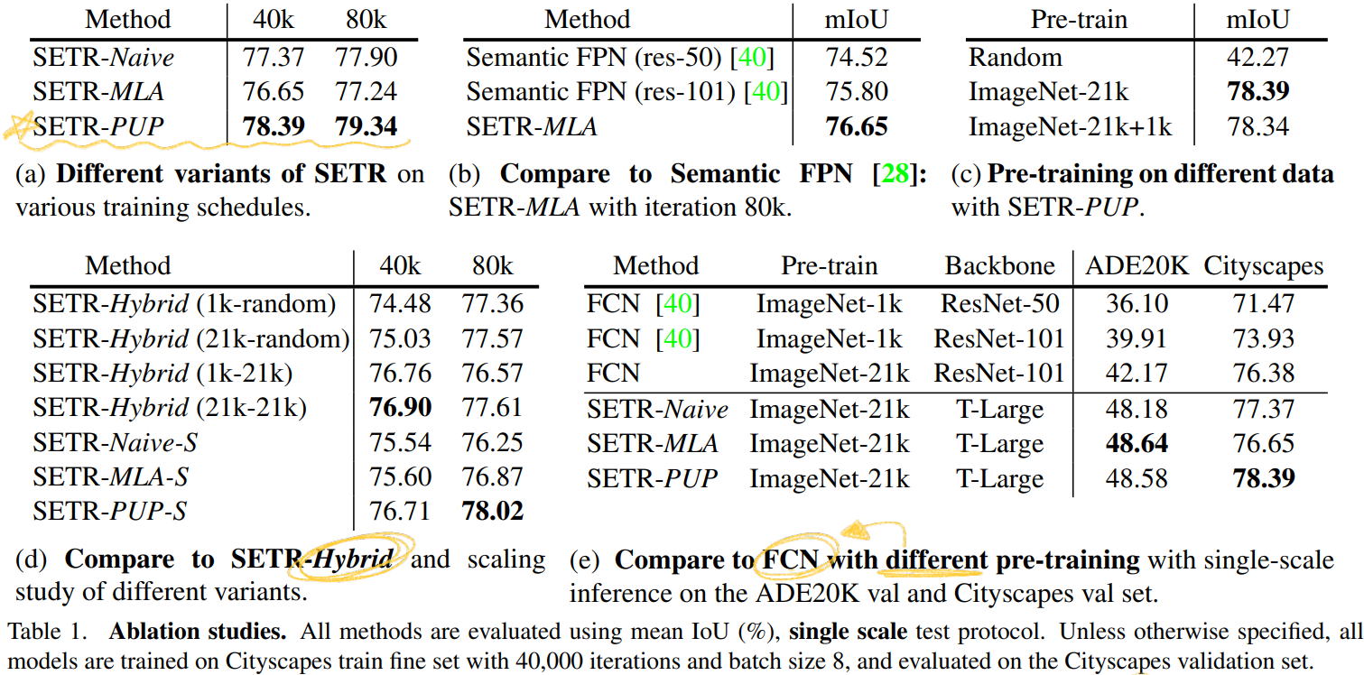
Ablation Studies
SOTA comparision